No one should have the impression that people who do molecular simulation only care about the Lennard-Jones fluid. It has been and continues to be an important test-bed for theories of the liquid state and phase-equilibria. Nevertheless, molecular simulation has been performed on a wide variety of materials.
As a single example, consider silicon. Perhaps the earliest attempt to
use molecular simulation to study a realistic atomic-scale model of
silicon was due to Stillinger and Weber [16]. I ``cut
my teeth'' on the Stillinger-Weber potential coding up my first real
research code in graduate school. I now make a version of that code
available to the students in this course, available at
mdswsi.c. This
code computes in reduced units as well; ![]() = 0.20951 nm,
= 0.20951 nm,
![]() = 2.1678 eV, and
= 2.1678 eV, and ![]() = 28.085 amu, which are appropriate
for a system of pure silicon. One reduced unit of temperature,
= 28.085 amu, which are appropriate
for a system of pure silicon. One reduced unit of temperature,
![]() , corresponds to 25156.73798 K.
, corresponds to 25156.73798 K.
The main reason to introduce Stillinger-Weber silicon here is to give
you an example of a three-body potential. Silicon forms 4-coordinated
tetrahedral bonded structures. The object of the three-body component
of the potential is to enforce the tetrahedral bond angle
(109.47![]() ) among triplets of bonded atoms.
) among triplets of bonded atoms.
The total potential is expressed as two sums, one for unique pair interactions, and another for unique triplet interactions:
| (220) |
The two-body models the bonds:
![\begin{displaymath}
v_2 \left(r\right) = \left\{\begin{array}{ll}
\epsilon A \l...
...t], & \mbox{$r < a$}\\
0 & \mbox{$r\ge a$}
\end{array}\right.
\end{displaymath}](img644.png) |
(221) |
The three body models the angles, and is the sum of functions of each
of the three angles of a triplet, ![]() :
:
| (222) |
Here I have employed the shorthand notation
![]() . Note that, in the
notation of this potential,
. Note that, in the
notation of this potential, ![]() is subtended at
is subtended at ![]() , and
, and
![]() :
:
 |
(223) |
One computes the angle-![]() term,
term, ![]() , and the angle-
, and the angle-![]() term,
term, ![]() , by permuting the indices appropriately.
, by permuting the indices appropriately.
The parameters used in the original study by Stillinger and Weber are:
| (224) | |||
| (225) | |||
| (226) | |||
| (227) | |||
| (228) | |||
| (229) | |||
| (230) |
As in any MD simulation, one computes the force on any particle ![]() from the negative gradient of the total potential:
from the negative gradient of the total potential:
| (231) | |||
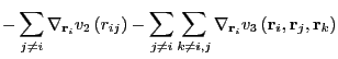 |
(232) |
The two-body term for the ![]() -
-![]() interaction is only slightly more
complicated than Lennard-Jones, due to the smooth cutoff. Here,
assuming
interaction is only slightly more
complicated than Lennard-Jones, due to the smooth cutoff. Here,
assuming ![]() and
and ![]() are within interaction range (
are within interaction range (![]() ), we
have for the force on
), we
have for the force on ![]() due to
due to ![]() :
:
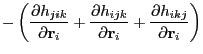
It is comparatively much more tedious to evaluate the three-body gradients.
Each of the partials in Eq. 241 is unique:
We can investigate what happens when we willfully ignore the three-body terms. Let us initialize atoms on a diamond-cubic lattice (the minimal energy lattice of silicon); a snapshot appears below.
 |
|
|
% gcc -o mdswsi_no3 mdswsi.c -lm -lgsl
% gcc -o mdswsi mdswsi.c -DTHREEBODY -lm -lgsl
Note also that this code uses the Andersen thermostat by default, with a default value of
% mdswsi -nu 0 -ns 10001 -icf init.xyzturns off the thermostat, which is what I have done for this little demonstration.
Below we plot the instantaneous temperature vs. time-step (0.001
![]() ) for the two runs. Notice that the system with the 3-body
forces intact remains steady at
) for the two runs. Notice that the system with the 3-body
forces intact remains steady at ![]() 0.12, while the system
without 3-body forces simply ``melts,'' with
0.12, while the system
without 3-body forces simply ``melts,'' with ![]() approaching 20,000 K
A quick look at a configuration (not shown) reveals that there is no
longer any crystalline order; the system is now an amorphous blob of
silicon atoms. The lesson of this little demonstration is that one
must have three-body forces to stabilize a diamond-cubic lattice.
approaching 20,000 K
A quick look at a configuration (not shown) reveals that there is no
longer any crystalline order; the system is now an amorphous blob of
silicon atoms. The lesson of this little demonstration is that one
must have three-body forces to stabilize a diamond-cubic lattice.
 |
|
|
![$\displaystyle -\frac{\partial }{\partial{\bf r}_i} \left\{\epsilon A \left(Br_{ij}^{-p}-r_{ij}^{-q}\right)\exp\left[\left(r_{ij}-a\right)^{-1}\right]\right\}$](img674.png)
![$\displaystyle -\epsilon A \frac{{\bf r}_{ij}}{r_{ij}}\left(\left.\left[\frac{\p...
...)\right]\right\vert _{r_{ij}}\exp\left[\left(r_{ij}-a\right)^{-1}\right]\right.$](img675.png)
![$\displaystyle \left.\left(Br_{ij}^{-p}-r_{ij}^{-q}\right)\left.\left\{\frac{\pa...
...al r}\exp\left[\left(r-a\right)^{-1}\right]\right\}\right\vert _{r_{ij}}\right)$](img677.png)
![$\displaystyle v_2\frac{{\bf r}_{ij}}{r_{ij}}\left[\frac{pBr_{ij}^{-p-1}-qr_{ij}^{-q-1}}{Br_{ij}^{-p}-r_{ij}^{-q}} + \left(r_{ij}-a\right)^{-2}\right]$](img681.png)
![\begin{displaymath}
\begin{array}{lll}
\mbox{\raisebox{-0.5cm}{\includegraphics[...
...k}}\frac{1}{r_{ij}}\right)
\cos\theta_{jik}\right]
\end{array}\end{displaymath}](img690.png)
![\begin{displaymath}
\begin{array}{lll}
\mbox{\raisebox{-0.5cm}{\includegraphics[...
...}}{r_{ij}}\frac{1}{r_{ij}}
\cos\theta_{ijk}\right]
\end{array}\end{displaymath}](img691.png)
![\begin{displaymath}
\begin{array}{lll}
\mbox{\raisebox{-0.5cm}{\includegraphics[...
...}}{r_{ik}}\frac{1}{r_{ik}}
\cos\theta_{ikj}\right]
\end{array}\end{displaymath}](img692.png)