So, we see now that, using the factorization trick, we have two
ensembles to average over:
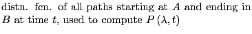 |
(302) | ||
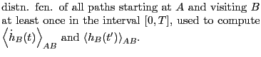 |
(303) |
We can compute averages in these two ensembles by MC sampling. A new
path is generated from an old path, and is accepted or rejected based
on a detailed balance criterion. Now, we sample these two path ensembles
in two different simulations, but the acceptance rules and trial moves
are the same. Let's generall call
![]() the
probability of path
the
probability of path ![]() . We start with an old path ``
. We start with an old path ``![]() '' and attempt
to generate a new path ``
'' and attempt
to generate a new path ``![]() ''. The acceptance rule obeying detailed
balance is
''. The acceptance rule obeying detailed
balance is
| (304) |
![]() is the a priori probabilit
of attemptying to generate
is the a priori probabilit
of attemptying to generate ![]() . The moves used in transition path
sampling MC guarantee
. The moves used in transition path
sampling MC guarantee
![]() . So,
. So,
| (305) |
So, what are the moves? There are two basic moves we can consider here.
It seems the real trick is generating an initial path of length
![]() that successfully connects region
that successfully connects region ![]() with region
with region ![]() . This can
be done with traditional MD by beginning a trajectory in state
. This can
be done with traditional MD by beginning a trajectory in state ![]() and
simply waiting long enough for it to cross into
and
simply waiting long enough for it to cross into ![]() . This might be
possible, but could easily be prohibitively expensive. A better
technique is to guess a path by creating a configuration which you
hypothesize to be a transition state, and then integrating
forward and backward in time to generate a path. It is accepted as an
initial path if the beginning lands in
. This might be
possible, but could easily be prohibitively expensive. A better
technique is to guess a path by creating a configuration which you
hypothesize to be a transition state, and then integrating
forward and backward in time to generate a path. It is accepted as an
initial path if the beginning lands in ![]() and the end in
and the end in ![]() .
.