The Metropolis Monte Carlo Method

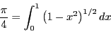
Monte Carlo is in general a technique for performing numerical integration. Consider the following integral:

$$I = \int_a^b f\left(x\right) dx$$ (57)

Now imagine that we have a second function, $\rho(x)$, which is positive in the interval $[a,b]$. We can also express $I$ as

$$I = \int_a^b \frac{f\left(x\right)}{\rho\left(x\right)}\rho\left(x\right) dx$$ (58)

If we think of $\rho\left(x\right)$ as a probability density, then what we have just expressed is the average of the quantity $f/\rho$ on $rho$ in the interval $[a,b]$:

$$I = \left<\frac{f\left(x\right)}{\rho\left(x\right)}\right>_\rho$$ (59)

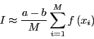
This implies that we can approximate $I$ by picking $M$ values $\left\{x_i\right\}$ randomly out of the probability distribution $\rho(x)$ and computing the following sum:

$$I \approx \frac{1}{M} \sum_{i=1}^{M} \frac{f\left(x_i\right)}{\rho\left(x_i\right)}$$ (60)

Note that this approximates the mean of $f/\rho$ as long as pick a large enough number of random numbers ($M$ is large enough) such that we ``densely'' cover the interval $[a,b]$. If $\rho\left(x\right)$ is uniform on $[a,b]$,

$$\rho\left(x\right) = \frac{1}{b-a}, a < x < b$$ (61)

and therefore,

$$I \approx \frac{a-b}{M} \sum_{i=1}^{M} f\left(x_i\right)$$ (62)

The next question is, how good an approximation is this, compared with more traditional one-dimensional numerical integration techniques, such as Simpson's rule and quadrature? A better phrasing of this question is, how expensive is this technique for a given level of accuracy, compared to traditional techniques? Consider this means to compute $\pi$:

$$\frac{\pi}{4} = \int_0^1 \left(1-x^2\right)^{1/2}dx$$ (63)

Allen and Tildesley [2] mention that, in order use Eq. 62 to compute $\pi$ to an accuracy of one part in 10$^6$ requires $M$ = 10$^7$ random values of $x_i$, whereas Simpson's rule required three orders of magnitude fewer points to discretize the interval to obtain an accuracy of one part in 10$^7$. So the answer is, integral estimation using uniform random variates is expensive.

But, the situation changes radically when the dimensionality of the integral is large, as is the case for an ensemble average. For example, for 100 particles having 300 coordinates, the configurational average $\left<G\right>$ (Eq. 54) could be discretized using Simpson's rule. If we did that, requesting only a modest 10 points per axis in configurational space, we would need to evaluate the integrand $Ge^{-\beta\mathscr{U}}$

10$^{300}$

times. This is an almost unimaginably large number (a googul cubed). Using a direct numerical technique to compute statistical mechanical averages is simply out of the question.

We therefore return to the idea of evaluating the integrand at a discrete set of points selected randomly from a distribution. Here we call upon the idea of importance sampling. Let us try to use whatever we know ahead of time about the integrand in picking our random distribution, $rho$, such that we minimize the number of points (i.e., the expense) necessary to give an estimate of $\left<G\right>$ to a given level of accuracy.

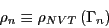
Now, clearly the states that contribute the most to the integrals we wish to evaluate by configurational averaging are those states with large Boltzmann factors; that is, those states for which $\rho_{NVT}$ is large. It stands to reason that if we randomly select points from $\rho_{NVT}$, we will do a pretty good job approximating the integral. So what we end up computing is the ``average of $G\rho_{NVT}$ over $\rho_{NVT}$'':

$$\left<G\rho_{NVT}/\rho_{NVT}\right> \approx \left<G\right>,$$ (64)

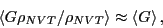
which should give an excellent approximation for $\left<G\right>$. The idea of using the $\rho_{NVT}$ as the sampling distribution is due to Metropolis et al. [6]. This makes the real work in computing $\left<G\right>$ generating states that randomly sample $\rho_{NVT}$.

Metropolis et al. [6] showed that an efficient way to do this involves generating a Markov chain of states which is constructed such that its limiting distribution is $\rho_{NVT}$. A Markov chain is just a sequence of trials, where (i) each trial outcome is a member of a finite set called ``state space,'' and (ii) every trial outcome depends only on the outcome that immediately precedes it. By ``limiting distribution,'' we mean that the trial acceptance probabilities are tuned such that the probability of observing the Markov chain atop a particular state is defined by some equilibrium probability distribution, $rho$. For the following discussion, it will be convenient to denote a particular state $n$ using $\Gamma_n$, instead of $\nu$.

A trial is some perturbation (usually small) of the coordinates specifying a state. For example, in an Ising system, this might mean flipping a randomly selected spin. In a system of particles in continuous space, it might mean displacing a randomly selected particle by a small amount $\delta r$ in a randomly chosen direction. There is a large variety of such ``trial moves'' for any particular system; we will only deal with a few simple ones in this course.

The probability that a trial move results in a successful transition from state $n$ to $m$ is denoted $\pi_{nm}$ and ${\bf\pi}$ is called the ``transition matrix.'' It must be specified ahead of time to execute a traditional Markov chain. Since the probability that a trial results in a successful transition to any state, the rows of ${\bf\pi}$ add to unity:

$$\sum_i \pi_{ni} = 1$$ (65)

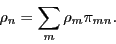
With this specification, we term ${\bf\pi}$ a ``stochastic'' matrix. Furthermore, for an equilibrium ensemble of states in state space, we require that transitions from state to state do not alter state weights as determined by the limiting distribution. So the weight of state $n$:

$$\rho_n \equiv \rho_{NVT}\left(\Gamma_n\right)$$ (66)

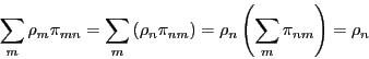
must be the result of transitions from all other states to state $n$:

$$\rho_n = \sum_m \rho_m \pi_{mn}.$$ (67)

For all states $n$, we can write Eq. 67 as a post-op matrix equation:

$${\bf\rho\pi} = {\bf\rho}$$ (68)

where ${\bf\rho}$ is the row vector of all state weights. Eq. 68 constrains our choice of ${\bf\pi}$. This means there is still more than one way to specify ${\bf\rho}$. Metropolis et al. [6] suggested:

$$\rho_m\pi_{mn} = \rho_n\pi_{nm}$$ (69)

That is, the probability of transitioning from state $m$ to $n$ is exactly equal to the probability of transitioning from state $n$ to $m$. This is called the ``detailed balance'' condition, and it guarantees that the state weights remain static. Observe:

$$\sum_m \rho_m\pi_{mn} = \sum_m\left(\rho_n\pi_{nm}\right) = \rho_n\left(\sum_m\pi_{nm}\right) = \rho_n$$ (70)

Detailed balance is, however, overly restrictive; this fact is of little importance in this course.

Metropolis et al. [6] chose to construct ${\bf\pi}$ as

$$\pi_{nm} = \alpha_{nm} {\rm acc}\left(n\rightarrow m\right)$$ (71)

where $\alpha$ is the probability that a trial move is attempted, and ${\rm acc}$ is the probability that a move is accepted. If the probability of proposing a move from $n$ to $m$ is equal to that of proposing a move from $m$ to $n$, then $\alpha_{nm} = \alpha_{mn}$, and the detailed balance condition is written:

$$\rho_n{\rm acc}\left(n\rightarrow m\right) = \rho_m{\rm acc}\left(m\rightarrow n\right)$$ (72)

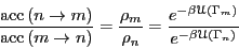
from which follows

$$\frac{{\rm acc}\left(n\rightarrow m\right)}{{\rm acc}\left(m... ...(\Gamma_m\right)}}{e^{-\beta\mathscr{U}\left(\Gamma_n\right)}}$$ (73)

giving

$$\frac{{\rm acc}\left(n\rightarrow m\right)}{{\rm acc}\left(m... ...]\right\} \equiv \exp\left(-\beta\Delta\mathscr{U}_{nm}\right)$$ (74)

where we have defined the change in potential energy as

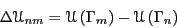$$\Delta\mathscr{U}_{nm} = \mathscr{U}\left(\Gamma_m\right)-\mathscr{U}\left(\Gamma_n\right)$$ (75)

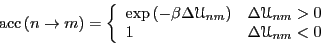
There are many choices for ${\rm acc}\left(n \rightarrow m\right)$ that satisfy Eq. 74. The original choice of Metropolis is used most frequently:

$${\rm acc}\left(n \rightarrow m\right) = \left\{\begin{array}... ...m} > 0\\ 1 & \Delta\mathscr{U}_{nm} < 0 \end{array} \right.$$ (76)

So, suppose we have some initial configuration $n$ with potential energy $U_n$. We make a trial move, temporarily generating a new configuration $m$. Now we calculate a new energy, $U_m$. If this energy is lower than the original, ($U_m < U_n$) we unconditionally accept the move, and configuration $m$ becomes the current configuration. If it is greater than the original, ($U_m > U_n$) we accept it with a probability consistent with the fact that the states both belong to a canonical ensemble. How does one in practice decide whether to accept the move? One first picks a uniform random variate $x$ on the interval $[0,1]$. If $x \le {\rm acc}\left(n \rightarrow m\right)$, the move is accepted.

The next section is devoted to an implementation of the Metropolis Monte Carlo method for a 2D Ising magnet.