- ...
cycles. 1
- Note that I have unceremoniously changed my
definition of ``cycle''. Before, one ``cycle'' was
 moves; now it
is a single move. This distinction isn't important for now, but I
thought you'd like to be made aware.
moves; now it
is a single move. This distinction isn't important for now, but I
thought you'd like to be made aware.
.
.
.
.
.
.
.
.
.
.
.
.
.
.
.
.
.
.
.
.
.
.
.
.
.
.
.
.
.
.
- ...
as2
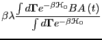
- Eq. 270 is a result of the following general
relations, given in Appendix C. For some quantity
 of a system
subject to a small constant perturbation,
of a system
subject to a small constant perturbation,  , the average of
the response of after the perturbation is removed,
, the average of
the response of after the perturbation is removed,
 , is given by
 |
(266) |
 is the trajectory of in the unperturbed system, and
 is shorthand for phase space point
 .
.
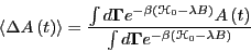
 is generally a function of , but not time. In the limit
as
is generally a function of , but not time. In the limit
as
 , and assuming that
 = 0, we
see that
= 0, we
see that
.
.
.
.
.
.
.
.
.
.
.
.
.
.
.
.
.
.
.
.
.
.
.
.
.
.
.
.
.
.
- ...,3
- If that second equality
in Eq. 279 looks fishy, but it is due to the fact that the time origin is chosen arbitrarily. For any autocorrelation function
.
.
.
.
.
.
.
.
.
.
.
.
.
.
.
.
.
.
.
.
.
.
.
.
.
.
.
.
.
.
- ... 2.0. 4
- Note that the code tps provided by F&S
(written by the eminent Thijs
Vlugt) is hard-coded with a path
length
 = 5
= 5  . To change to 2 , we edit the file
maxarray.inc, and change the parameter Maxtraject from
1000 to 400. This is the number of ``slices'' in a trajectory, and
each slice is Nshort = 5 time steps. The reason = 5 was
originally used is likely because the exercise for which this code was
originally written was conducted with a total energy of 9
. To change to 2 , we edit the file
maxarray.inc, and change the parameter Maxtraject from
1000 to 400. This is the number of ``slices'' in a trajectory, and
each slice is Nshort = 5 time steps. The reason = 5 was
originally used is likely because the exercise for which this code was
originally written was conducted with a total energy of 9  vs. the 15 we consider here; that is, we run at a higher
effective temperature. Dellago's original paper considered = 9
particles with a total energy of 9 , so we should be running
at the same effective temperature as Dellago with the larger number of
particles considered by Vlugt. We are, however, running at a slightly
lower density (
vs. the 15 we consider here; that is, we run at a higher
effective temperature. Dellago's original paper considered = 9
particles with a total energy of 9 , so we should be running
at the same effective temperature as Dellago with the larger number of
particles considered by Vlugt. We are, however, running at a slightly
lower density (
 ) than considered by Dellago
(
) than considered by Dellago
(
 ).
).
.
.
.
.
.
.
.
.
.
.
.
.
.
.
.
.
.
.
.
.
.
.
.
.
.
.
.
.
.
.
- ...-vectors. 5
- One
modification of this code is a necessary one: the implementation of
the real-space energy was left as an exercise. Other modifications
made easily include embedding the main program inside a double loop
over desired
 and
and  values.
.
.
.
.
.
.
.
.
.
.
.
.
.
.
.
.
.
.
.
.
.
.
.
.
.
.
.
.
.
.
- ...eq:dos). 6
- Strictly speaking, the density of states has
units of
 , because
 is the number of states with energy between
  and
and  . However,
in common usage in the literature, the quantity
. However,
in common usage in the literature, the quantity  is
referred to as the density of states, although it is correctly termed
the microcanonical partition function.
is
referred to as the density of states, although it is correctly termed
the microcanonical partition function.
.
.
.
.
.
.
.
.
.
.
.
.
.
.
.
.
.
.
.
.
.
.
.
.
.
.
.
.
.
.