Band Excitation Piezoresponse Force Microscopy of \(PbZr_{0.2}Ti_{0.8}O_3\)#
Film grown and measurements conducted by Joshua C. Agar at Oak Ridge National Laboratory
This dataset has been the subject of 4 manuscripts:
Agar, J., Damodaran, A. R., Pandya, S., C, Cao, Y., Vasudevan, R. K., Xu, R., Saremi, S., Li, Q., Kim, J., McCarter, M. R., Dedon, L. R., Angsten, T., Balke, N., Jesse, S., Asta, M., Kalinin, S. V. & Martin, L. W. Three-State Ferroelastic Switching and Large Electromechanical Responses in PbTiO3 Thin Films. Adv. Mater. 29, 1702069 (2017). doi:10.1002/adma.201702069
Agar, J. C., Cao, Y., Naul, B., Pandya, S., van der Walt, S., Luo, A. I., Maher, J. T., Balke, N., Jesse, S., Kalinin, S. V., Vasudevan, R. K. & Martin, L. W. Machine detection of enhanced electromechanical energy conversion in PbZr0.2Ti0.8O3 thin films. Adv. Mater. 30, e1800701 (2018). doi:10.1002/adma.201800701
Griffin, L. A., Gaponenko, I. & Bassiri-Gharb, N. Better, Faster, and Less Biased Machine Learning: Electromechanical Switching in Ferroelectric Thin Films. Adv. Mater. e2002425 (2020). doi:10.1002/adma.202002425
Qin, S., Guo, Y., Kaliyev, A. T. & Agar, J. C. Why it is Unfortunate that Linear Machine Learning ‘Works’ so well in Electromechanical Switching of Ferroelectric Thin Films. Adv. Mater. e2202814 (2022). doi:10.1002/adma.202202814
Import Packages#
import h5py
import numpy as np

import matplotlib.pyplot as plt
from matplotlib.patches import ConnectionPatch


from m3_learning.nn.random import random_seed
from m3_learning.viz.style import set_style
from m3_learning.be.util import print_be_tree
from m3_learning.be.processing import convert_amp_phase, fit_loop_function, SHO_Fitter, SHO_fit_to_array, loop_lsqf
from m3_learning.viz.layout import layout_fig
from m3_learning.util.h5_util import make_dataset, make_group
from m3_learning.util.file_IO import download_and_unzip
from scipy.signal import resample
from scipy import fftpack


set_style("default")
random_seed(seed=42)

%matplotlib inline
default set for seaborn
default set for matplotlib
Pytorch seed was set to 42
Numpy seed was set to 42
tensorflow seed was set to 42
Loading data for SHO fitting#
path = r"./"
url = 'https://zenodo.org/record/7297755/files/data_file.h5?download=1'
filename = 'data_file.h5'
save_path = './'

download_and_unzip(filename, url, save_path)
Using files already downloaded
Prints the Tree to show the Data Structure
print_be_tree(path + "data_file.h5")
/
├ Measurement_000
  ---------------
  ├ Channel_000
    -----------
    ├ Bin_FFT
    ├ Bin_Frequencies
    ├ Bin_Indices
    ├ Bin_Step
    ├ Bin_Wfm_Type
    ├ Excitation_Waveform
    ├ Noise_Floor
    ├ Position_Indices
    ├ Position_Values
    ├ Raw_Data
    ├ Raw_Data-SHO_Fit_000
      --------------------
      ├ Fit
      ├ Guess
      ├ Guess-Loop_Fit_000
        ------------------
        ├ Fit
        ├ Fit_Loop_Parameters
        ├ Guess
        ├ Guess_Loop_Parameters
        ├ Loop_Metrics
        ├ Loop_Metrics_Indices
        ├ Loop_Metrics_Values
        ├ Projected_Loops
        ├ completed_fit_positions
        ├ completed_guess_positions
      ├ Spectroscopic_Indices
      ├ Spectroscopic_Values
      ├ completed_fit_positions
      ├ completed_guess_positions
    ├ Spatially_Averaged_Plot_Group_000
      ---------------------------------
      ├ Bin_Frequencies
      ├ Max_Response
      ├ Mean_Spectrogram
      ├ Min_Response
      ├ Spectroscopic_Parameter
      ├ Step_Averaged_Response
    ├ Spatially_Averaged_Plot_Group_001
      ---------------------------------
      ├ Bin_Frequencies
      ├ Max_Response
      ├ Mean_Spectrogram
      ├ Min_Response
      ├ Spectroscopic_Parameter
      ├ Step_Averaged_Response
    ├ Spectroscopic_Indices
    ├ Spectroscopic_Values
    ├ UDVS
    ├ UDVS_Indices
    ├ complex
      -------
      ├ imag
      ├ real
    ├ magn_spec
      ---------
      ├ amp
      ├ phase
├ Raw_Data-SHO_Fit_000
  --------------------
  ├ Fit
  ├ Guess
  ├ Spectroscopic_Indices
  ├ Spectroscopic_Values
  ├ completed_fit_positions
  ├ completed_guess_positions
Datasets and datagroups within the file:
------------------------------------
/
/Measurement_000
/Measurement_000/Channel_000
/Measurement_000/Channel_000/Bin_FFT
/Measurement_000/Channel_000/Bin_Frequencies
/Measurement_000/Channel_000/Bin_Indices
/Measurement_000/Channel_000/Bin_Step
/Measurement_000/Channel_000/Bin_Wfm_Type
/Measurement_000/Channel_000/Excitation_Waveform
/Measurement_000/Channel_000/Noise_Floor
/Measurement_000/Channel_000/Position_Indices
/Measurement_000/Channel_000/Position_Values
/Measurement_000/Channel_000/Raw_Data
/Measurement_000/Channel_000/Raw_Data-SHO_Fit_000
/Measurement_000/Channel_000/Raw_Data-SHO_Fit_000/Fit
/Measurement_000/Channel_000/Raw_Data-SHO_Fit_000/Guess
/Measurement_000/Channel_000/Raw_Data-SHO_Fit_000/Guess-Loop_Fit_000
/Measurement_000/Channel_000/Raw_Data-SHO_Fit_000/Guess-Loop_Fit_000/Fit
/Measurement_000/Channel_000/Raw_Data-SHO_Fit_000/Guess-Loop_Fit_000/Fit_Loop_Parameters
/Measurement_000/Channel_000/Raw_Data-SHO_Fit_000/Guess-Loop_Fit_000/Guess
/Measurement_000/Channel_000/Raw_Data-SHO_Fit_000/Guess-Loop_Fit_000/Guess_Loop_Parameters
/Measurement_000/Channel_000/Raw_Data-SHO_Fit_000/Guess-Loop_Fit_000/Loop_Metrics
/Measurement_000/Channel_000/Raw_Data-SHO_Fit_000/Guess-Loop_Fit_000/Loop_Metrics_Indices
/Measurement_000/Channel_000/Raw_Data-SHO_Fit_000/Guess-Loop_Fit_000/Loop_Metrics_Values
/Measurement_000/Channel_000/Raw_Data-SHO_Fit_000/Guess-Loop_Fit_000/Projected_Loops
/Measurement_000/Channel_000/Raw_Data-SHO_Fit_000/Guess-Loop_Fit_000/completed_fit_positions
/Measurement_000/Channel_000/Raw_Data-SHO_Fit_000/Guess-Loop_Fit_000/completed_guess_positions
/Measurement_000/Channel_000/Raw_Data-SHO_Fit_000/Spectroscopic_Indices
/Measurement_000/Channel_000/Raw_Data-SHO_Fit_000/Spectroscopic_Values
/Measurement_000/Channel_000/Raw_Data-SHO_Fit_000/completed_fit_positions
/Measurement_000/Channel_000/Raw_Data-SHO_Fit_000/completed_guess_positions
/Measurement_000/Channel_000/Spatially_Averaged_Plot_Group_000
/Measurement_000/Channel_000/Spatially_Averaged_Plot_Group_000/Bin_Frequencies
/Measurement_000/Channel_000/Spatially_Averaged_Plot_Group_000/Max_Response
/Measurement_000/Channel_000/Spatially_Averaged_Plot_Group_000/Mean_Spectrogram
/Measurement_000/Channel_000/Spatially_Averaged_Plot_Group_000/Min_Response
/Measurement_000/Channel_000/Spatially_Averaged_Plot_Group_000/Spectroscopic_Parameter
/Measurement_000/Channel_000/Spatially_Averaged_Plot_Group_000/Step_Averaged_Response
/Measurement_000/Channel_000/Spatially_Averaged_Plot_Group_001
/Measurement_000/Channel_000/Spatially_Averaged_Plot_Group_001/Bin_Frequencies
/Measurement_000/Channel_000/Spatially_Averaged_Plot_Group_001/Max_Response
/Measurement_000/Channel_000/Spatially_Averaged_Plot_Group_001/Mean_Spectrogram
/Measurement_000/Channel_000/Spatially_Averaged_Plot_Group_001/Min_Response
/Measurement_000/Channel_000/Spatially_Averaged_Plot_Group_001/Spectroscopic_Parameter
/Measurement_000/Channel_000/Spatially_Averaged_Plot_Group_001/Step_Averaged_Response
/Measurement_000/Channel_000/Spectroscopic_Indices
/Measurement_000/Channel_000/Spectroscopic_Values
/Measurement_000/Channel_000/UDVS
/Measurement_000/Channel_000/UDVS_Indices
/Measurement_000/Channel_000/complex
/Measurement_000/Channel_000/complex/imag
/Measurement_000/Channel_000/complex/real
/Measurement_000/Channel_000/magn_spec
/Measurement_000/Channel_000/magn_spec/amp
/Measurement_000/Channel_000/magn_spec/phase
/Raw_Data-SHO_Fit_000
/Raw_Data-SHO_Fit_000/Fit
/Raw_Data-SHO_Fit_000/Guess
/Raw_Data-SHO_Fit_000/Spectroscopic_Indices
/Raw_Data-SHO_Fit_000/Spectroscopic_Values
/Raw_Data-SHO_Fit_000/completed_fit_positions
/Raw_Data-SHO_Fit_000/completed_guess_positions

The main dataset:
------------------------------------
<HDF5 file "data_file.h5" (mode r+)>

The ancillary datasets:
------------------------------------
<HDF5 dataset "Position_Indices": shape (3600, 2), type "<u4">
<HDF5 dataset "Position_Values": shape (3600, 2), type "<f4">
<HDF5 dataset "Spectroscopic_Indices": shape (4, 63360), type "<u4">
<HDF5 dataset "Spectroscopic_Values": shape (4, 63360), type "<f4">

Metadata or attributes in a datagroup
------------------------------------
BE_actual_duration_[s] : 0.004
BE_amplitude_[V] : 1
BE_auto_smoothing : auto smoothing on
BE_band_edge_smoothing_[s] : 4832.1
BE_band_edge_trim : 0.094742
BE_band_width_[Hz] : 200000
BE_bins_per_band : 0
BE_center_frequency_[Hz] : 1310000
BE_desired_duration_[s] : 0.004
BE_phase_content : chirp-sinc hybrid
BE_phase_variation : 1
BE_points_per_BE_wave : 0
BE_repeats : 4
FORC_V_high1_[V] : 1
FORC_V_high2_[V] : 10
FORC_V_low1_[V] : -1
FORC_V_low2_[V] : -10
FORC_num_of_FORC_cycles : 1
FORC_num_of_FORC_repeats : 1
File_MDAQ_version : MDAQ_VS_090915_01
File_date_and_time : 18-Sep-2015 18:32:14
File_file_name : SP128_NSO
File_file_path : C:\Users\Asylum User\Documents\Users\Agar\SP128_NSO\
File_file_suffix : 99
IO_AO_amplifier : 10
IO_AO_range_[V] : +/- 10
IO_Analog_Input_1 : +/- .1V, FFT
IO_Analog_Input_2 : off
IO_Analog_Input_3 : off
IO_Analog_Input_4 : off
IO_DAQ_platform : NI 6115
IO_rate_[Hz] : 4000000
VS_amplitude_[V] : 16
VS_cycle_fraction : full
VS_cycle_phase_shift : 0
VS_measure_in_field_loops : in and out-of-field
VS_mode : DC modulation mode
VS_number_of_cycles : 2
VS_offset_[V] : 0
VS_read_voltage_[V] : 0
VS_set_pulse_amplitude[V] : 0
VS_set_pulse_duration[s] : 0.002
VS_step_edge_smoothing_[s] : 0.001
VS_steps_per_full_cycle : 96
data_type : BEPSData
grid_/single : grid
grid_contact_set_point_[V] : 1
grid_current_col : 1
grid_current_row : 1
grid_cycle_time_[s] : 10
grid_measuring : 0
grid_moving : 0
grid_num_cols : 60
grid_num_rows : 60
grid_settle_time_[s] : 0.15
grid_time_remaining_[h;m;s] : 10
grid_total_time_[h;m;s] : 10
grid_transit_set_point_[V] : 0.1
grid_transit_time_[s] : 0.15
num_bins : 165
num_pix : 3600
num_udvs_steps : 384
SHO Fitting#
Note: this code takes around 15 minutes to execute
SHO_Fitter(path + "data_file.h5")
Extract Data#
# Opens the data file
h5_f = h5py.File(path + "data_file.h5", "r+")

# number of samples per SHO fit
num_bins = h5_f["Measurement_000"].attrs["num_bins"]

# number of pixels in the image
num_pix = h5_f["Measurement_000"].attrs["num_pix"]

# number of pixels in x and y dimensions
num_pix_1d = int(np.sqrt(num_pix))

# number of DC voltage steps
voltage_steps = h5_f["Measurement_000"].attrs["num_udvs_steps"]

# sampling rate
sampling_rate = h5_f["Measurement_000"].attrs["IO_rate_[Hz]"]

# BE bandwidth
be_bandwidth = h5_f["Measurement_000"].attrs["BE_band_width_[Hz]"]

# BE center frequency
be_center_frequency = h5_f["Measurement_000"].attrs["BE_center_frequency_[Hz]"]

# Frequency Vector in Hz
frequency_bin = h5_f["Measurement_000"]["Channel_000"]["Bin_Frequencies"][:]

# Resampled frequency vector
wvec_freq = resample(frequency_bin, 80)

# extracting the excitation waveform
be_waveform = h5_f["Measurement_000"]["Channel_000"]["Excitation_Waveform"]

# extracting spectroscopic values
spectroscopic_values = h5_f["Measurement_000"]["Channel_000"]["Spectroscopic_Values"]

# get raw data (real and imaginary combined)
raw_data = h5_f["Measurement_000"]["Channel_000"]["Raw_Data"]
Saves the Data#
shape = h5_f["Measurement_000"]["Channel_000"]["Raw_Data"].shape

#creates the necessary structure in the H5_file
make_group(h5_f["Measurement_000"]["Channel_000"], 'complex')
make_group(h5_f["Measurement_000"]["Channel_000"], 'magn_spec')
make_dataset(h5_f["Measurement_000"]["Channel_000"]['complex'], 'real', np.real(h5_f["Measurement_000"]["Channel_000"]["Raw_Data"]))
make_dataset(h5_f["Measurement_000"]["Channel_000"]['complex'], 'imag', np.imag(h5_f["Measurement_000"]["Channel_000"]["Raw_Data"]))

amp, phase = convert_amp_phase(raw_data)

make_dataset(h5_f["Measurement_000"]["Channel_000"]['magn_spec'], 'amp', amp)
make_dataset(h5_f["Measurement_000"]["Channel_000"]['magn_spec'], 'phase', phase)
could not add group - it might already exist
could not add group - it might already exist
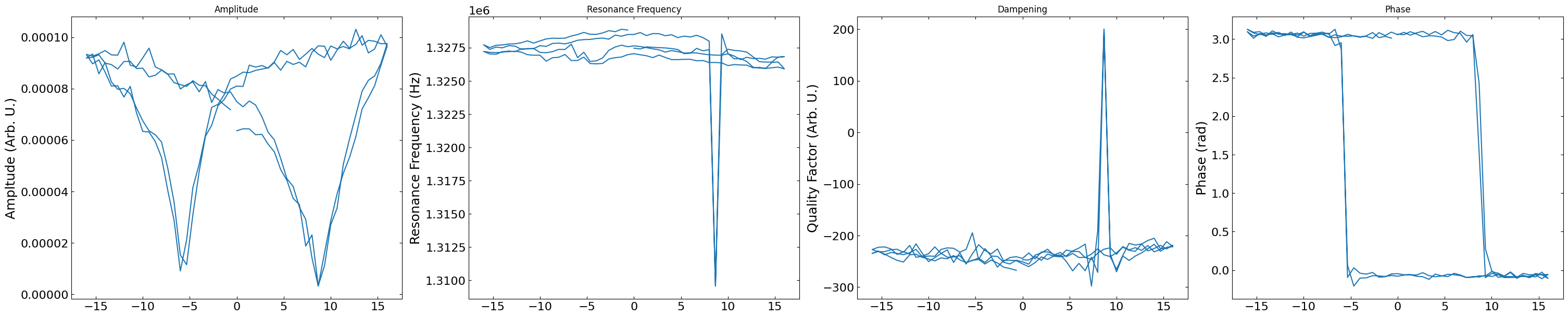
Plots the SHO Fit Results#
dc_voltage = h5_f["Measurement_000"]["Channel_000"]['Raw_Data-SHO_Fit_000']['Spectroscopic_Values'][0,1::2]
SHO_fit_results = SHO_fit_to_array(h5_f["Measurement_000"]["Channel_000"]["Raw_Data-SHO_Fit_000"]["Fit"])
pix = np.random.randint(0,3600)

figs, ax = layout_fig(4, 4, figsize=(30, 6))

labels = [{'title': "Amplitude",
            'y_label': "Ampltude (Arb. U.)"},
         {'title': "Resonance Frequency",
            'y_label': "Resonance Frequency (Hz)"},
         {'title': "Dampening",
            'y_label': "Quality Factor (Arb. U.)"},
        {'title': "Phase",
            'y_label': "Phase (rad)"}]

for i, ax in enumerate(ax):
    ax.plot(dc_voltage, SHO_fit_results[pix,1::2,i])
    ax.set_title(labels[i]['title'])
    ax.set_ylabel(labels[i]['y_label'])
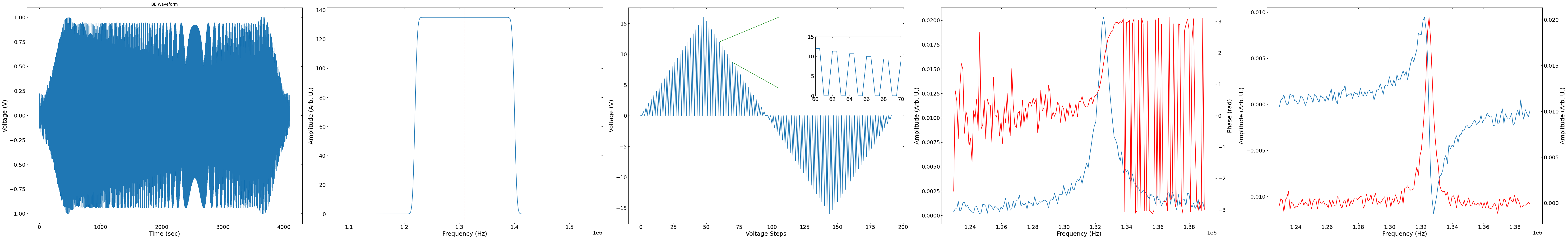
Visualize Raw Data#
# Selects a random point and timestep to plot
pixel = np.random.randint(0,h5_f["Measurement_000"]["Channel_000"]['magn_spec']['amp'][:].shape[0])
timestep = np.random.randint(h5_f["Measurement_000"]["Channel_000"]['magn_spec']['amp'][:].shape[0]/num_bins)

print(pixel, timestep)
fig, ax = layout_fig(5, 5, figsize=(6 * 11, 10))

be_timesteps = len(be_waveform) / 4
print("Number of time steps: " + str(be_timesteps))
ax[0].plot(be_waveform[: int(be_timesteps)])
ax[0].set(xlabel="Time (sec)", ylabel="Voltage (V)")
ax[0].set_title("BE Waveform")

resonance_graph = np.fft.fft(be_waveform[: int(be_timesteps)])
fftfreq = fftpack.fftfreq(int(be_timesteps)) * sampling_rate
ax[1].plot(
    fftfreq[: int(be_timesteps) // 2], np.abs(resonance_graph[: int(be_timesteps) // 2])
)
ax[1].axvline(
    x=be_center_frequency,
    ymax=np.max(resonance_graph[: int(be_timesteps) // 2]),
    linestyle="--",
    color="r",
)
ax[1].set(xlabel="Frequency (Hz)", ylabel="Amplitude (Arb. U.)")
ax[1].set_xlim(
    be_center_frequency - be_bandwidth - be_bandwidth * 0.25,
    be_center_frequency + be_bandwidth + be_bandwidth * 0.25,
)

hysteresis_waveform = (
    spectroscopic_values[1, ::165][192:] * spectroscopic_values[2, ::165][192:]
)
x_start = 120
x_end = 140

ax[2].plot(hysteresis_waveform)
ax_new = fig.add_axes([0.52, 0.6, 0.3/5.5, 0.25])
ax_new.plot(np.repeat(hysteresis_waveform, 2))
ax_new.set_xlim(x_start, x_end)
ax_new.set_ylim(0, 15)
ax_new.set_xticks(np.linspace(x_start, x_end, 6))
ax_new.set_xticklabels([60, 62, 64, 66, 68, 70])
fig.add_artist(
    ConnectionPatch(
        xyA=(x_start // 2, hysteresis_waveform[x_start // 2]),
        coordsA=ax[2].transData,
        xyB=(105, 16),
        coordsB=ax[2].transData,
        color="green",
    )
)
fig.add_artist(
    ConnectionPatch(
        xyA=(x_end // 2, hysteresis_waveform[x_end // 2]),
        coordsA=ax[2].transData,
        xyB=(105, 4.5),
        coordsB=ax[2].transData,
        color="green",
    )
)
ax[2].set_xlabel("Voltage Steps")
ax[2].set_ylabel("Voltage (V)")

ax[3].plot(
    frequency_bin,
    h5_f["Measurement_000"]["Channel_000"]['magn_spec']['amp'][:].reshape(num_pix, -1, num_bins)[pixel, timestep],
)
ax[3].set(xlabel="Frequency (Hz)", ylabel="Amplitude (Arb. U.)")
ax2 = ax[3].twinx()
ax2.plot(
    frequency_bin,
    h5_f["Measurement_000"]["Channel_000"]['magn_spec']['phase'][:].reshape(num_pix, -1, num_bins)[pixel, timestep],
    "r",
)
ax2.set(xlabel="Frequency (Hz)", ylabel="Phase (rad)");

ax[4].plot(frequency_bin, h5_f["Measurement_000"]["Channel_000"]['complex']['real'][pixel].reshape(-1, num_bins)[timestep], label="Real")
ax[4].set(xlabel="Frequency (Hz)", ylabel="Amplitude (Arb. U.)")
ax3 = ax[4].twinx()
ax3.plot(
    frequency_bin, h5_f["Measurement_000"]["Channel_000"]['complex']['imag'][pixel].reshape(-1, num_bins)[timestep],'r', label="Imaginary")
ax3.set(xlabel="Frequency (Hz)", ylabel="Amplitude (Arb. U.)");
3507 14
Number of time steps: 4096.0
/home/ferroelectric/anaconda3/envs/STEM/lib/python3.9/site-packages/matplotlib/cbook/__init__.py:1369: ComplexWarning: Casting complex values to real discards the imaginary part
  return np.asarray(x, float)
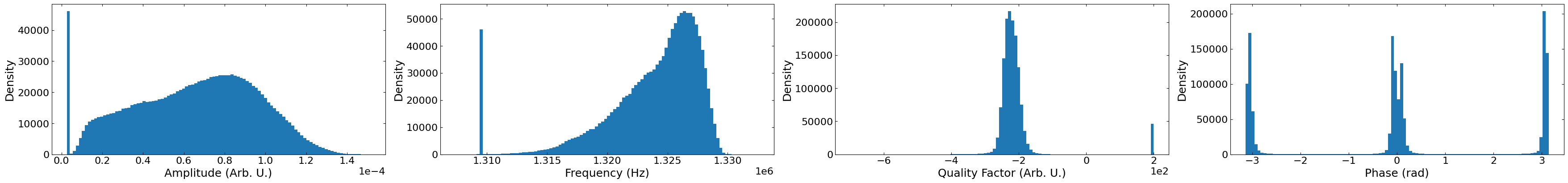
Visualize the SHO Fit Results#
# create a list for parameters
fit_results_list = []
for sublist in np.array(
    h5_f["Measurement_000"]["Channel_000"]["Raw_Data-SHO_Fit_000"]["Fit"]
):
    for item in sublist:
        for i in item:
            fit_results_list.append(i)

# flatten parameters list into numpy array
fit_results_list = np.array(fit_results_list).reshape(num_pix, voltage_steps, 5)
# check distributions of each parameter before and after scaling
fig, axs = layout_fig(4, 4, figsize=(35, 4))

units = [
    "Amplitude (Arb. U.)",
    "Frequency (Hz)",
    "Quality Factor (Arb. U.)",
    "Phase (rad)",
]

for i in range(4):
    axs[i].hist(fit_results_list[:, :, i].flatten(), 100)

i = 0
for i, ax in enumerate(axs.flat):
    ax.set(xlabel=units[i], ylabel="Density")
    ax.ticklabel_format(axis="x", style="sci", scilimits=(0, 0))
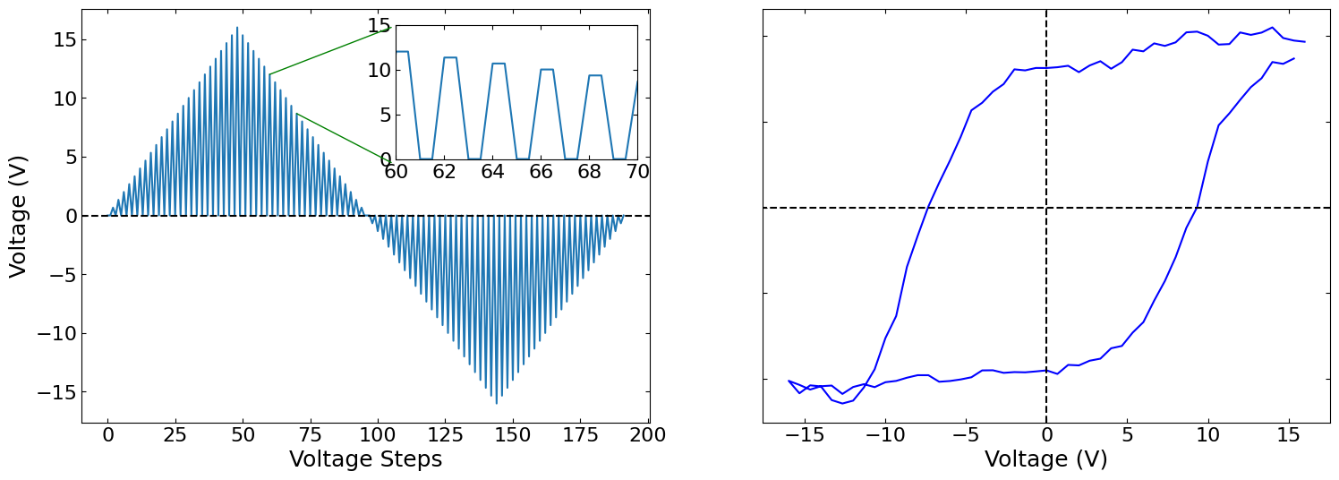
Piezoelectric Hysteresis Loops#
h5_main = h5_f["Measurement_000"]["Channel_000"]["Raw_Data-SHO_Fit_000"]["Guess"]
h5_loop_fit, h5_loop_group = fit_loop_function(h5_f, h5_main)
Consider calling test() to check results before calling compute() which computes on the entire dataset and writes results to the HDF5 file

Note: Loop_Fit has already been performed with the same parameters before. These results will be returned by compute() by default. Set override to True to force fresh computation

[<HDF5 group "/Measurement_000/Channel_000/Raw_Data-SHO_Fit_000/Guess-Loop_Fit_000" (11 members)>]

Note: Loop_Fit has already been performed with the same parameters before. These results will be returned by compute() by default. Set override to True to force fresh computation

[<HDF5 group "/Measurement_000/Channel_000/Raw_Data-SHO_Fit_000/Guess-Loop_Fit_000" (11 members)>]
Returned previously computed results at /Measurement_000/Channel_000/Raw_Data-SHO_Fit_000/Guess-Loop_Fit_000
/home/ferroelectric/anaconda3/envs/STEM/lib/python3.9/site-packages/pyUSID/io/hdf_utils/simple.py:888: UserWarning: A dataset named: Guess_Loop_Parameters already exists in group: /Measurement_000/Channel_000/Raw_Data-SHO_Fit_000/Guess-Loop_Fit_000
  warn('A dataset named: {} already exists in group: {}'.format(dset_name, h5_group.name))
/home/ferroelectric/anaconda3/envs/STEM/lib/python3.9/site-packages/pyUSID/io/hdf_utils/simple.py:888: UserWarning: A dataset named: Fit_Loop_Parameters already exists in group: /Measurement_000/Channel_000/Raw_Data-SHO_Fit_000/Guess-Loop_Fit_000
  warn('A dataset named: {} already exists in group: {}'.format(dset_name, h5_group.name))
# Formats the data for viewing
proj_nd_shifted = loop_lsqf(h5_f)
proj_nd_shifted_transposed = np.transpose(proj_nd_shifted, (1, 0, 2, 3))
No spectroscopic datasets found as attributes of /Measurement_000/Channel_000/Position_Indices
No position datasets found as attributes of /Measurement_000/Channel_000/Raw_Data-SHO_Fit_000/Spectroscopic_Values
fig, axs = plt.subplots(figsize=(18, 6), nrows=1, ncols=2)
hysteresis_waveform = (
    spectroscopic_values[1, ::165][192:] * spectroscopic_values[2, ::165][192:]
)
x_start = 120
x_end = 140

axs[0].plot(hysteresis_waveform)
ax_new = fig.add_axes([0.32, 0.6, 0.15, 0.25])
ax_new.plot(np.repeat(hysteresis_waveform, 2))
ax_new.set_xlim(x_start, x_end)
ax_new.set_ylim(0, 15)
ax_new.set_xticks(np.linspace(x_start, x_end, 6))
ax_new.set_xticklabels([60, 62, 64, 66, 68, 70])
fig.add_artist(
    ConnectionPatch(
        xyA=(x_start // 2, hysteresis_waveform[x_start // 2]),
        coordsA=axs[0].transData,
        xyB=(105, 16),
        coordsB=axs[0].transData,
        color="green",
    )
)
fig.add_artist(
    ConnectionPatch(
        xyA=(x_end // 2, hysteresis_waveform[x_end // 2]),
        coordsA=axs[0].transData,
        xyB=(105, 4.5),
        coordsB=axs[0].transData,
        color="green",
    )
)
axs[0].set_xlabel("Voltage Steps")
axs[0].set_ylabel("Voltage (V)")

i = np.random.randint(0, num_pix_1d, 2)
axs[1].plot(dc_voltage[24:120], proj_nd_shifted_transposed[i[0], i[1], :, 3], "blue")
axs[1].ticklabel_format(axis="y", style="sci", scilimits=(0, 0))
axs[1].set(xlabel="Voltage (V)", ylabel="Amplitude (Arb. U.)")
axs[1].label_outer()

axs[0].axhline(y=0, xmax=200, linestyle="--", color="black")
axs[1].axhline(y=0, xmin=-16, xmax=16, linestyle="--", color="black")
axs[1].axvline(x=0, linestyle="--", color="black")
<matplotlib.lines.Line2D at 0x7fbe293cb130>
# Closes the h5_file
h5_f.close()