6.2 Thermodynamic Integration

Thermodynamic integration is a conceptually simple, albeit expensive, way to calculate free energy differences from MC or MD simulations. In this example, we will consider the calculation (again) of chemical potential in a Lennard-Jones fluid at a given temperature and density, a task performed very well already by the Widom method (so long as the densities are not too high.) More details of the method can be found in Reference [15].

We begin with the relation derived in the book for a free energy difference, \(F_{II} - F_{I}\), between two systems which are identical (same number of particles, density, temperature, etc.) except that they obey two different potentials. System I obeys \(\mathscr {U}_I\) and System II \(\mathscr {U}_{II}\). To measure this free energy difference, we must integrate along a reversible path from I to II. So let us suppose that we can write a “metapotential” that uses a switching parameter, \(\lambda \), to measure distance along this path. So, when \(\lambda = 0\), we are in System I, and when \(\lambda = 1\) we are in System II. One way we might encode this (though this is not necessarily a general splitting, as we shall see below) is \begin{equation} \mathscr {U}\left (\lambda \right ) = \left (1-\lambda \right )\mathscr {U}_{I} + \lambda \mathscr {U}_{II} \end{equation}

Let us consider the canonical partition function for a system obeying a general potential \(\mathscr {U}\left (\lambda \right )\): \begin{equation} Q\left (N,V,T,\lambda \right ) = \frac {1}{\Lambda ^{3N}N!}\int d{\bf r}^N\exp \left [-\beta \mathscr {U}\left (\lambda \right )\right ] \end{equation} Recalling that the free energy is given by \(F = -k_BT\ln Q\), we can express the derivative of the Helmholtz free energy with respect to \(\lambda \): \begin{equation} \begin {aligned} \left (\frac {\partial F\left (\lambda \right )}{\partial \lambda }\right )_{N,V,T} & = -\frac {1}{\beta }\frac {\partial }{\partial \lambda }\ln Q\left (N,V,T,\lambda \right ) \\ & = -\frac {1}{\beta Q\left (N,V,T,\lambda \right )}\frac {\partial Q\left (N,V,T,\lambda \right )}{\partial \lambda } \\ & = \frac { \int d{\bf r}^N \left (\partial \mathscr {U}\left (\lambda \right )/\partial \lambda \right )\exp \left [-\beta \mathscr {U}\left (\lambda \right )\right ]}{ \int d{\bf r}^N\exp \left [-\beta \mathscr {U}\left (\lambda \right )\right ]} \end {aligned} \end{equation}

The free energy difference between I and II is given by: \begin{equation} F_{II} - F{I} = \int _{\lambda =0}^{\lambda =1}\left \langle \frac {\partial \mathscr {U}}{\partial \lambda }\right \rangle _\lambda d\lambda \end{equation} where, \(\left \langle \frac {\partial \mathscr {U}}{\partial \lambda }\right \rangle _\lambda \) is the ensemble average of the derivative of \(\mathscr {U}\) with respect to \(\lambda \).

To compute \(\mu _{\rm ex}\), we imagine two systems: System I has \(N-1\) “real” particles, and 1 ideal gas particle, and system II has \(N\) real particles. The two free energies can be written: \begin{equation} \begin {aligned} F_{\rm I} & = F_{\rm id}\left (N,V,T\right ) + F_{\rm ex}\left (N-1,V,T\right ) \\ F_{\rm II} & = F_{\rm id}\left (N,V,T\right ) + F_{\rm ex}\left (N,V,T\right ) \end {aligned} \end{equation}

For large values of \(N\), we see that \(\mu _{\rm ex} = F_{\rm II} - F_{\rm I}\). So, we have another route to compute \(\mu _{\rm ex}\). First, we tag a particle \(i_\lambda \), call it the “\(\lambda \)-particle”, and apply the following modified potential to its pairwise interactions: \begin{equation} \label {eq:lambda_lj} U_{\rm LJ,\lambda }\left (r;\lambda \right ) = 4\left (\lambda ^5r^{-12} - \lambda ^3r^{-6}\right ) \end{equation} So, the total potential is given by \begin{equation} \mathscr {U} = {\sum _{i<j}} ^\prime U_{\rm LJ}\left (r_{ij}\right ) + \sum _i U_{\rm LJ,\lambda }\left (r_{i,i_\lambda };\lambda \right ) \end{equation} where the prime denotes that we ignore particle \(i_\lambda \) in the sum. When \(\lambda = 1\), all particles interact fully, and we have System II.

Next, we conduct many independent MC simulations at various values of \(\lambda \) and a given value of \(\rho \) and \(T\), generating for each \(\left (T,\rho \right )\) a table of \(\left \langle \partial \mathscr {U}/\partial \lambda \right \rangle _\lambda \) vs. \(\lambda \) which can be integrated to yield a single value for \(\mu _{\rm ex}\). This turns out to be an expensive way to compute the chemical potential for a Lennard-Jones fluid, compared to the Widom method (Sec. 6.1), for at least low to moderate densities.

I have done a rough comparison of the thermodynamic integration method described above to the grand canonical MC simulation technique described in Sec. 5.1. Below is a plot of \(\left \langle \partial \mathscr {U}/\partial \lambda \right \rangle _\lambda \) vs. \(\lambda \) for three densities \(\rho \in \left \{0.5, 0.7, 0.9\right \}\). Each point is computed from a single MC simulation using the code mclj_ti.c. The temperature was \(T\) = 2.0, and run for 10\(^6\) cycles for \(N\) = 216. We see that the data is not terribly smooth; it is not clear how many more cycles would result in smoother data.

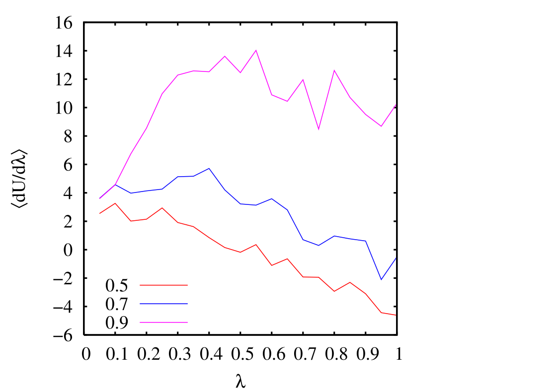
However, integration is not too sensitive to these fluctuations. As we see below, integrating each of these curves to produce a single value of \(\mu _{\rm ex}\) produces values that are not too off from the grand canonical simulations.

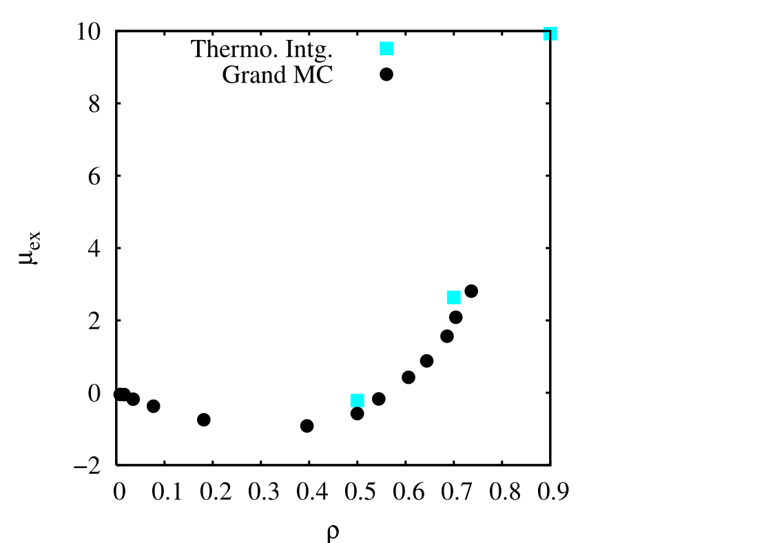
The grand canonical simulations are of course much cheaper, as it requires only a single MC simulation to give a value of \(\mu _{\rm ex}\). However, thermodynamic integration is a generally applicable technique for computing free energy differences.

Questions:

1. Can we make the agreement better by running more MC cycles? How about by using more values of \(\lambda \)?
2. How does this compare to the Widom method?