7.4 Densities of States: The Wang-Landau Monte Carlo Method

One of the most interesting recent developments in molecular simulation are the so-called “density of states” methods, first implemented by Wang and Landau [22, 23]. In principle, these techniques provide a route to calculating the density of states of a system of interest, \(\Omega (E)\) (Eq. 19). ⁶ Determining \(\Omega \) gives a full understanding of the thermodynamics of a system, because the entropy is calculable directly as \begin{equation} S = k_BT\ln \Omega \end{equation} So, it is not undesirable at all to be able to compute \(\Omega \).

Now, we know that \(\Omega \) is buried in the probability distribution of energy that arises from standard NVT Monte Carlo simulation: \begin{equation} P(E) = \Omega (E)\exp \left (-\beta E\right )\left /\sum _{i}\Omega (E_i)\exp \left (-\beta E_i\right )\right . \end{equation} If we run a simple NVT MC simulation and populate a histogram of total energy, \(H(E)\), we can in principle compute \(\Omega (E)\) by first normalizing \(H(E)\) \(\rightarrow P(E)\) and multiplying each entry \(i\) by the factor \(\exp \left (+\beta E_i\right )\). The problem in practice is that states for which the Boltzmann factor (\(\exp \left (-\beta E_i\right )\)) is low are rarely if ever visited in reasonable time, and the statistical strength of \(H(E)\) in such regions of energy is therefore poor. Indeed, conventional MC is designed to not cover all of energy space, but to perform importance sampling of configurational space. Furthermore, if the Markov process is trapped in a local minimum on the potential energy hypersurface, barrier states with vanishingly small Boltzmann factors effectively prevent the escape of the process, preventing an adequate sampling of the potential energy hypersurface. For these reasons, it is desirable to perform a random walk in energy rather than configurational space.

In this section, we’ll review the two papers by Wang and Landau which introduced their technique by demonstrating how to compute \(\Omega \) for Ising and Potts systems by conducting random walks in energy space. These are lattice systems; more recent work has been focused on developing efficient continuous-space versions of the technique (E.g., [24, 25]).

7.4.1 The Algorithm

The Wang-Landau algorithm is a method which converges upon \(\Omega (E)\) to within a given tolerance. First, we must understand what energy levels are accessible to our system; let us call this set \(\left \{E_i: i=1,\dots ,N_e\right \}\), where \(N_e\) is the number of levels. Let us imagine conducting a random walk in energy space such that the observed histogram of visited levels, \(H(E)\), is uniform, or “flat.” This random walk must be guided by some underlying probability distribution, \(\mathscr {N}\), which tells us whether to accept or reject a proposed step, \(o\rightarrow n\), in the walk. Generally, \(\mathscr {N}\) is incorporated in a Metropolis acceptance rule: \begin{equation} \label {eq:acc1} {\rm acc}(o\rightarrow n) = \min \left (1,\frac {\mathscr {N}(n)}{\mathscr {N}(o)}\right ) \end{equation} By conditionally accepting trials based on Eq. 274, we guarantee that \(\mathscr {N}\) is a static equilibrium distribution (assuming our trial moves obey detailed balance, or the balance condition is met in some other way). Now, if \(\mathscr {N}\) is the canonical distribution, the probability of observing a particular energy level, \(E_i\), is proportional to \(\exp \left (-E_i/k_BT\right )\).

Now consider that each energy level has \(\Omega (E_i)\) allowable microstates, each with the same probability, \(1/\Omega (E_i)\), by the fundamental hypothesis. The probability of observing the system in energy level \(E_i\) is the composite probability of observing it in one of the microstates with energy \(E_i\). If we want the probability of observing the system in energy level \(E_i\) to be uniform, then the probability of observing any particular microstate should be proportional to \(1/\Omega (E_i)\). So, the probability distribution we should use is \begin{equation} \mathscr {N} \propto 1/\Omega (E_i), \end{equation} and the acceptance rule becomes: \begin{equation} \label {eq:acc2} {\rm acc}(o\rightarrow n) = \min \left (1,\frac {\Omega (o)}{\Omega (n)}\right ) \end{equation}

Now, here is why we want to construct a flat histogram. If we can, then we know that have the “correct” \(\Omega \). But we don’t know \(\Omega \) to begin with. So now we need a way to begin with a guess for \(\Omega \) and then systematically refine it until we achieve a flat histogram in energy space. An efficient technique for successively refining a guess for \(\Omega \) from a sequence of Monte-Carlo simulations was the major contribution of Wang and Landau. [22, 23]

In this algorithm, we start with the initial guess \(\Omega (E) = 1\), and the histogram is initialized as \(H(E) = 0\). Then, we begin making trial moves and accepting or rejecting based on the acceptance rule in Eq. 276. After a move, we find ourselves in energy state \(E_i\), and we update both the histogram and the density of states: \begin{equation} \begin {aligned} H(E_i) & \rightarrow H(E_i) + 1 \\ \Omega (E_i) & \rightarrow f\Omega (E_i) \end {aligned} \end{equation} Note that this is done regardless of whether we wind up in state \(E_i\) due to an accepted move or a rejected move. The density of states update factor, \(f\), begins at a relatively large value (\(f = e^1 = 2.718281828\)). The updates continue until the histogram is “sufficiently flat.” At this point, the histogram is reset to 0, and \(f\) is reduced according to \begin{equation} \label {eq:wl:f_update} f \rightarrow \sqrt {f} \end{equation} Then, the simulation continues again until the histogram is sufficiently flat. After several iterations, \(f\) gets closer and closer to 1, and changes to \(\Omega \) become smaller and smaller. The series of runs is terminated after \(\ln f\) is about 10\(^{-8}\).

By “sufficiently flat,” Wang and Landau suggest that the histogram is such that the bin with the minimum number of hits is within 95% of the mean number of hits per bin. This is a particularly strong criterion, and more recent work suggests that it is adequate to require merely that each bin has a minimum number of hits, regardless of the mean value [26].

The factor update relation (Eq. 278) is also somewhat arbitrary. What is required is that \(f\) approach unity in a scheduled manner. A more general rule might be \begin{equation} f \rightarrow \sqrt [n]{f}\ \ \ \ n \ge 2 \end{equation}

It is important to note that, because the acceptance rule is changing during the simulation, detailed balance is not strictly obeyed. However, it is very close to being obeyed when \(f\approx 1\). How does one choose a proper initial value and update scheme for \(f\)? There is unfortunately no general guidance on this in the current literature, other than the original realization of Wang and Landau that too large a value of \(f\) introduces large statistical fluctuations in \(\Omega \) which might become “frozen in,” while too small a value for \(f\) will require much too many visits to produce a flat histogram.

Also, the magnitude of \(\Omega \) is normally such that we can’t tabulate it directly; it is advantageous instead to tabulate its log. So the array used to store \(\Omega \) actually stores \(\ln \Omega \), and the update of a bin becomes: \begin{equation} \ln \Omega \rightarrow \ln \Omega + \ln f \end{equation} The acceptance rule does not change, of course; it is simply reformulated as \begin{equation} {\rm acc}(o\rightarrow n) = \min \left [1,\exp \left (\ln \Omega (o)-\ln \Omega (n)\right )\right ] \end{equation}

Finally, because the acceptance rule involves a ratio of probabilities, \(\Omega \) is not determined absolutely, but rather to within a constant factor. Unless we know the exact \(\Omega \) for some reference state (as we do for certain lattice models, such at the Ising magnet and the Potts glass), we cannot obtain absolute thermal quantities (entropy and free energies) from the \(\Omega \) obtained using this method. This is usually not a problem, either because we can “pin down” \(\Omega \) at a known reference, or because we don’t care about absolutes, but only differences.

7.4.2 A Conventional MC Study of the \(Q\) = 10 Potts Model

An impressive example of the power of the WL method appears in the latter of the two original WL papers [23]. Here, the object of study is the Potts model [27]. This is an \(L\times L\) lattice of \(N\) sites (i.e., \(N = L^2\)) where each site can have a spin value, \(q_i\), between 1 and \(Q\). WL considered the ten-state model; \(Q\) = 10. The Hamiltonian of the Potts model is \begin{equation} \mathscr {H} = -\sum _{\left \langle ij\right \rangle }\delta \left (q_i,q_j\right ) \end{equation} where the sum is over all nearest neighbor pairs.

Under periodic boundary conditions, the ground state energy of the Potts model is given by \begin{equation} E_0 = -2L^2 \end{equation} and the density of states at \(E_0\) (i.e., the degeneracy of the ground state) is easily seen to be \begin{equation} \Omega (E_0) = Q. \end{equation} The \(N\) energy levels are \begin{equation} -E_0,-E_0+8,-E_0+12,\dots ,-4,0,4,\dots ,E_0-12,E_0-8,E_0 \end{equation} The ten-state Potts model displays a first-order phase transition with a critical temperature of \(T_c = 0.701232\) in the thermodynamic limit (\(N\rightarrow \infty \)). The two coexisting phases are characterized by an average energy per particle of -0.965 and -1.671, respectively.

First, let’s conduct normal NVT sampling of a ten-state, \(L\) = 12 Potts model at temperatures well below, near, and well-above the critical temperature. (The dual purpose code wl-w.c can accomplish this.) At precisely the critical temperature, we should see two peaks of equal height in the energy histogram. Our trial move will consist of randomly selecting one of the 144 spins and then randomly selecting a spin value between 1 and 10. Below, I show the histograms of energy per spin after 10\(^6\) cycles (one cycle = 144 attempted flips) for various temperatures, all begun from the same initial (randomly assigned) configuration which is initially in the high-energy regime (E/N \(\approx \) -0.25). (\(T\) = 0.70991 is the critical temperature, \(T_c\), for the \(L\) = 12, \(Q\) = 10 Potts model as calculated by Wang and Landau.)

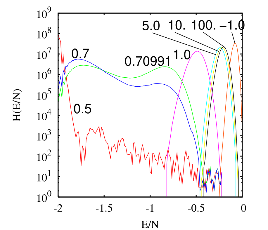
Notice that precisely pinpointing \(T_c\) using a series of NVT MC simulations (if we assume that 10\(^6\) cycles is enough – I have not yet claimed that it is) would be extremely difficult. For \(T\) = 0.7, the peaks are not of equal height, but an increase of a mere 0.0991 brings them to the same height (the signature of a critical temperature). How would we know how to zoom in on \(T\) = 0.70991? It is conceivable that we could embed NVT MC inside some nonlinear optimization routine whose objective function is a measure of relative peak heights, which must be minimized by allowing \(T\) to vary. This could be automated and could in principle provide a very accurate \(T_c\) after a finite number of runs. But we don’t know ahead of time how many runs would be required, nor if our optimization scheme is efficient enough to allow us to find \(T_c\) to some tolerable level of precision in a reasonable time.

Now, imagine that we could in some way compute the density of states, \(\Omega (E)\), from a single simulation. We could then easily arrive at an estimate for \(T_c\) by simply evaluating canonical energy histograms at various \(T\), each constructed from \(\Omega (E)\), until we find one for which the peak heights are the same. Consider: \begin{equation} \label {eq:canonical_histogram} H(E/N) \propto \Omega (E)\exp \left (-E/k_BT\right ). \end{equation}

Can we compute \(\Omega (E)\) from an NVT MC simulation? In principle, yes. We could rearrange Eq. 286: \begin{equation} \label {eq:anti_boltz} H(E/N)\exp \left (+\beta E\right ) \propto \Omega (E) \end{equation} This certainly suggests that if we run NVT MC, tabulate a histogram of energy states, and the postmultiply it by the “anti-Boltzmann” factor \(\exp \left (+\beta E\right )\), we will recover \(\Omega (E)\). But the data from the 10\(^6\)-cycle MC runs shown in the above figure kills any hope of being able to do this in practice. You can see that none of the histograms cover the entire domain of accessible energy levels, so we cannot use any single histogram to produce \(\Omega (E)\). You can also see that the very highest energy levels are not accessed even at extremely high temperatures. (Interestingly, a negative temperature resolves this part of the energy spectrum quite well; this indicates that the entropy of the Potts model for \(E > -0.25\) decreases with increasing energy.) The histogram taken at the lowest temperature appears to cover a broad part of the domain, but most of it is covered with very poor statistical accuracy, as evidenced by the large fluctuations. The histograms taken near the critical temperature of \(T\) = 0.70991 cover a relatively broad domain relatively well, so it is at least conceivable that we can produce part of \(\Omega (E)\) from these histograms.

The figure below shows the application of Eq. 287 to determine partial densities of states for each histogram shown in the previous figure.

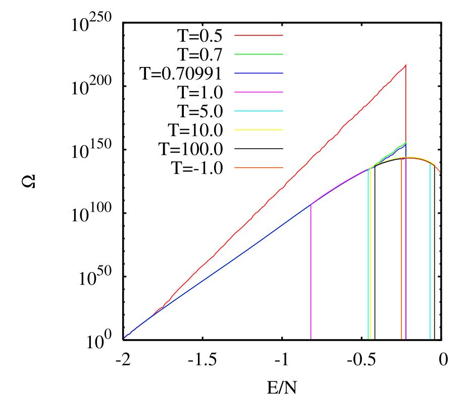
From this data, we can see the trace of the curve defining the true density of states. It appears to have a maximum at \(E/M\approx -0.25\) of a whopping 10\(^{145}\) states. We also see that the density of states decreases with energy for \(E/N > -0.25\); energy levels higher than this are apparently sampled well in an MC run with negative temperature. Now, in order to piece the true \(\Omega (E)\) together from these many runs, we took advantage of the fact that \(\Omega (E_0) = Q\), and scaled the densities to have them match in the overlapping regions. Notice that the two partial densities of states for \(T\) = 0.7 and 0.70991 agree (not surprising), but that the density of states for \(T\) = 0.5 appears much too large. All told, it appears that the total curve is adequately represented by the anti-Boltzmann-treated histograms from just three 10\(^6\)-cycle NVT MC runs: \(T \in \left \{0.7,1.0,-1.0\right \}\).

Now, I have to admit that I have cheated somewhat. I knew ahead of time that the density of states has a maximum, so I knew that negative temperature MC would resolve some part of it. I also knew that the critical temperature is 0.70991, but it was nice to see that number supported by standard MC. Let us now learn how to compute \(\Omega \) from a single MC run using the Wang-Landau technique.

7.4.3 The Potts Model treated by Wang-Landau MC

Now we will use the WL algorithm to compute \(\Omega (E)\) for the \(L\) = 12 ten-state Potts model. (I used the code wl-w.c to obtain these results.) The relevant run parameters we have to specify are the exponent for the update rule of the factor \(f\), the initial and final values of \(f\), and the flatness criterion for the histogram. The data presented here are from a single run for which \(\ln f_{\rm initial}\) = 1, \(\ln f_{\rm final}\) = 10\(^{-8}\), and \(\ln f_{i+1} = \frac {1}{2}\ln f_{i}\); this prescribes a total of 26 independent values of \(f\) for which a random walk in energy space must be executed. A histogram is considered sufficiently flat if the minimum value if the histogram is greater than or equal to 80% of the mean value.

The figure below shows the resulting final \(\Omega (E)\), compared to the piecemeal \(\Omega (E)\) computed from three NVT MC simulations. We see that the two methods give essentially the same function.

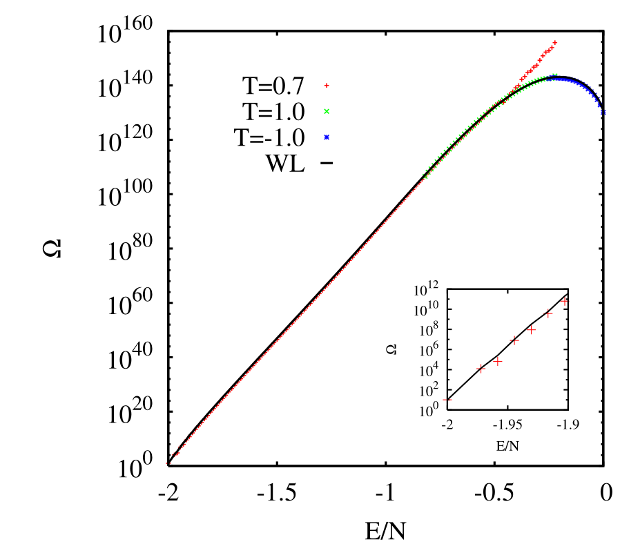
The close-up shown in the inset reveals some significant differences at the lowest energy levels between the WL and NVT results. This is because the visits to the lowest energy levels were quite rare in the MC case, making the statistical accuracy of the energy histogram in this subdomain poor.

The next figure shows the cumulative cost (in number of cycles) of the WL method for this system, and the relative error in neighboring estimates of \(\Omega \), as functions of the number of updates to the factor \(f\). The relative error is defined as \begin{equation} \epsilon \equiv \int dE \left (\ln \Omega _{i}-\ln \Omega _{i-1}\right )^2 \end{equation}

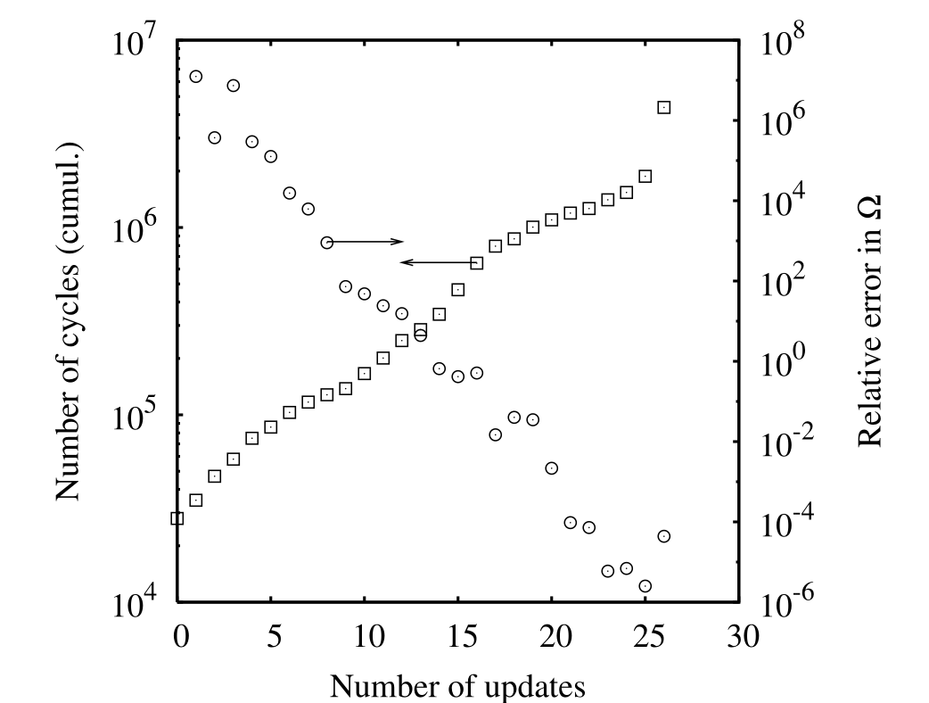
We see from this data that it requires roughly \(10^6\) cycles to converge \(\Omega \) to a tolerance of about 10\(^{-4}\), and that an additional \(3\times 10^6\) cycles does not improve this convergence. So, WL for this system is somewhat less expensive than the \(3\times 10^6\) required for the canonical MC runs.

Of course, the canonical MC runs would have been much more expensive had I not known ahead of time what the critical temperature was. For the WL method, no such knowledge is required a priori.

It should be pointed out that \(L\) = 12 is a very small system. Wang and Landau broke major new ground in studying the thermodynamics of the Potts model by considering \(L\) up to 200.

Although WL does arrive at an accurate estimate of \(\Omega \), it is not dramatically more efficient than conventional NVT MC. One of the reasons is due to the nature of the random walk: “steps” in energy space are necessarily local. Changing one spin changes energy by at most \(\pm \)4, and on average the change in energy per flip is much lower in absolute value than that. So the system can spend a lot of time trying to get away from a large subdomain of energy space for which the histogram is already sufficiently flat, in order to explore neighboring subdomains. WL showed that this deficiency can be partially avoided by conducting several parallel runs in different energy windows, which overlap a little bit to allow matching of the resulting densities of states.

7.4.4 How “flat” is “flat”?

In this section, we report results of a small case study which investigates the required flatness criterion to achieve a converged density of states. We will consider the converged \(\Omega \) computed using the 80% criterion as the “exact” result, and compare this to \(\Omega \)’s computed using the criterion that every bin in the energy histogram has at least \(M\) hits. We considered \(M \in \left \{2,20,200,2000,20000,200000\right \}\). In order to minimize the number of cycles, we will sample the histogram (that is, query its flatness) once per cycle. We also used the same termination criterion for the update of \(f\). In the figure below, I show both the relative error between \(\Omega \) computed with the \(M\)-criterion and \(\Omega _{\rm exact}\), as well as the number of cycles required for the \(M\)-criterion computation.

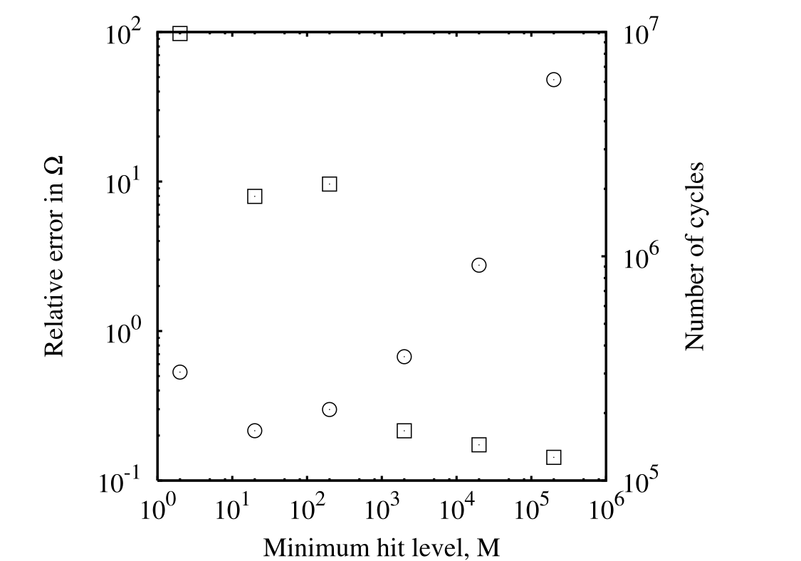
Interestingly, we see that even out to \(>10^6\) cycles, our result has only marginally converged to the exact result; an error of \(\approx 0.1\) is larger than the iteration-to-iteration convergence tolerance of \(\approx 10^{-4}\) observed in the original run. Nevertheless, this level of error is very small; the curves are indistinguishable on a plot. Another interesting fact is that the \(M\) = 2 run is apparently more expensive than the \(M\) = 20 run. This is likely due to fact that the initial configuration for each run segment (each value of \(f\)) is different; it is the final configuration from the previous segment. It just so happens that the 23rd iteration for \(M\) = 2 begins in a configuration that initiates a walk that more slowly covers energy space than the configurations in the \(M\) = 20 runs. Beyond \(M\) = 20, the behavior is as expected: increasing \(M\) makes the simulation more expensive.