7.2 Rare Events: Path-Sampling Monte Carlo

In this section, we will consider the technique of transition path sampling Monte Carlo simulation for calculating rate constants [17, 18]. This technique is one of many designed to overcome time-scale limitations in gathering statistics on processes driven by rare events, or thermally-activated transitions. When performed correctly, transition path sampling provides a means to gain a statistically significant understanding of reaction mechanisms. One of the most significant example uses of this technique is a recent prediction of rate constants for folding-like transitions in simulations of atomically specific protein fragments in explicit solvent [19].

The code used in this section was downloaded from Berend Smit’s Molecular Simulation course webpage.

7.2.1 Fundamentals

Consider a unimolecular isomerization reaction: \begin{equation} A~^{\stackrel {\textstyle k_{AB}}{\textstyle \rightharpoonup }}_{\stackrel {\textstyle \leftharpoondown }{\textstyle k_{BA}}}~B \end{equation} \(k_{AB}\) is the forward rate constant for the reaction, and \(k_{BA}\) is the backward rate constant. They are required to express the concentration balances for species \(A\) and \(B\) in the traditional way: \begin{equation} \begin {aligned} \frac {d C_A}{d t} & = -k_{AB}C_A + k_{BA}C_B \\ \frac {d C_B}{d t} & = k_{AB}C_A - k_{BA}C_B \end {aligned} \end{equation} At equilibrium, the time derivatives vanish, and \(C_A \rightarrow \left \langle C_A\right \rangle \), and \begin{equation} K = \frac {\left \langle C_A\right \rangle }{\left \langle C_B\right \rangle } = \frac {k_{BA}}{k_{AB}} \end{equation} We now ask, how does an initial perturbation in the concentration of \(A\), written \(\Delta A\), decay with time, assuming \(C_A + C_B = C\) = const.? \begin{equation} \begin {aligned} \frac {d \left (C_A + \Delta C_A\right )}{d t} & = -k_{AB}\left (C_A + \Delta C_A\right ) + k_{BA}\left (C_B - \Delta C_A\right ) \\ \frac {d C_A}{d t} & = -k_{AB}\Delta C_A - k_{BA}\Delta C_A = -\left (k_{AB}+k_{BA}\right )\Delta C_A \end {aligned} \end{equation} We can easily solve this to yield: \begin{equation} \label {eq:tps_macro1} \Delta C_A\left (t\right ) = \Delta C_A\left (0\right )\exp \left [-\left (k_{AB}+k_{BA}\right )t\right ] \equiv \Delta C_A\left (0\right )e^{-t/\tau _R} \end{equation} which defines the “decay time”: \begin{equation}\label {eq:tps_1} \begin {aligned} \tau _R &= \left (k_{AB} + k_{BA}\right )^{-1} \\ &= k_{AB}^{-1}\left (1+\frac {\left \langle C_A\right \rangle }{\left \langle C_B\right \rangle }\right )^{-1} \\ &= \frac {\left \langle C_B\right \rangle }{k_{AB}} \end {aligned} \end{equation} (The last equality assumes the concentrations are normalized such that \(C_A + C_B = 1\); that is, we can consider \(C_A\) as the probability of observing “state” \(A\).)

Now we make a connection to the microscopic. Imagine that the two states labelled \(A\) and \(B\) are separated from each other along some general reaction coordinate \(q\) which has a large free energy barrier at position \(q^*\):

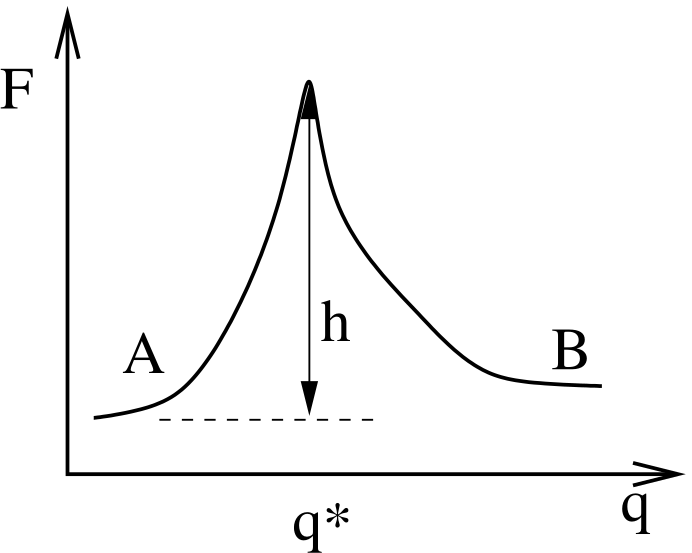
This is a free energy barrier because the system presumably has many more degrees of freedom other than (which may or may not contribute to) \(q\). Now, we enter the realm of linear response theory (See Appendix C in F&S), and ask, what is the behavior or the system with a finitely small, static perturbation toward state \(A\)? We express this as a perturbation Hamiltonian: \begin{equation} \mathscr {H} = \mathscr {H}_0 -\epsilon g_A\left (q-q^*\right ) \end{equation} where \(\mathscr {H}_0\) is the reference Hamiltonian of the unperturbed system. Here, \(g_A\) is an indicator function which is 1 if we are in state \(A\) and 0 otherwise: \begin{equation} g_A\left (x\right ) = \left \{\begin {array}{ll} 1 & \mbox {$x<0$}\\ 0 & \mbox {$x>0$} \end {array}\right . \end{equation} Notice that the peturbation lowers the energy by a little bit (\(\epsilon \)) when the system chooses to be in state \(A\). Here, we think of \(\epsilon \) as a switch we can flip in order to perturb the system. We measure the static pertubation as the difference between the average concentration of \(A\) in the perturbed state to that in the unperturbed state: \begin{equation} \Delta C_A = \left \langle C_A\right \rangle _\epsilon - \left \langle C_A\right \rangle _0 = \left \langle g_A\right \rangle _\epsilon - \left \langle g_A\right \rangle _0 \end{equation} Notice that because of our choice in magnitude for \(g_A\), we can consider its ensemble average, \(\langle g_A\rangle \), to be the probability of observing the system in state A, which is, due to our normalization of concentration, equivalent to the concentration of A.

Our first step is to find the linear response of \(\Delta C_A\) to \(\epsilon \), defined as \begin{equation} \left (\frac {\partial \Delta C_A}{\partial \epsilon }\right )_{\epsilon =0} = \left (\frac {\partial \left \langle g_A\right \rangle }{\partial \epsilon }\right )_{\epsilon =0} \end{equation} So let us first compute \(\langle g_A\rangle _\epsilon \) in the canonical ensemble: \begin{equation} \left \langle g_A\right \rangle _\epsilon = \frac { \int d{\bf q}^Nd{\bf p}^N \exp \left [-\beta \mathscr {H}_0\left ({\bf q},{\bf p}\right )+\beta \epsilon g_A\left (q-q^*\right )\right ]g_A\left (q-q^*\right )}{ \underbrace {\int d{\bf q}^Nd{\bf p}^N \exp \left [-\beta \mathscr {H}_0\left ({\bf q},{\bf p}\right )+\beta \epsilon g_A\left (q-q^*\right )\right ]}_{Z_\epsilon }} \end{equation} Here, we have defined \(Z_\epsilon \) as the unnormalized canonical partition function, merely to make the following gymnastics a little more transparent. Differentiating with respect to \(\epsilon \): \begin{equation} \frac {\partial \left \langle g_A\right \rangle _\epsilon }{\partial \epsilon } = \frac {1}{Z_\epsilon }\int d{\bf q}^Nd{\bf p}^N \exp \left (-\beta \mathscr {H}_0+\beta \epsilon g_A\right )\beta g_A^2 - \frac {1}{Z_\epsilon ^2}\left [\int d{\bf q}^Nd{\bf p}^N \exp \left (-\beta \mathscr {H}_0+\beta \epsilon g_A\right )g_A\right ]\left [\int d{\bf q}^Nd{\bf p}^N \exp \left (-\beta \mathscr {H}_0+\beta \epsilon g_A\right )\beta g_A\right ], \end{equation} which simplifies to \begin{equation} \frac {\partial \left \langle g_A\right \rangle _\epsilon }{\partial \epsilon } = \beta \left \langle g_A^2\right \rangle _\epsilon - \beta \left \langle g_A\right \rangle ^2_\epsilon . \end{equation} At \(\epsilon =0\) this gives the remarkable result \begin{equation} \left (\frac {\partial \Delta C_A}{\partial \epsilon }\right )_{\epsilon =0} = \beta \left (\left \langle g_A^2\right \rangle _0 - \left \langle g_A\right \rangle _0^2\right ). \end{equation}

Now, we haven’t said anything in detail about the structure of \(g_A\), but in fact, to perform this analysis, we require that it be continuous through the origin. But, we can make it vary from 1 to 0 across as narrow a region of \(q\) around the origin as we like. Then it is true that, at all values of \(q\) except perhaps right at the barrier position \(q^*\), \begin{equation} g_A^2 = g_A \ \ \ \mbox {so\ \ \ } \left \langle g_A^2\right \rangle = \left \langle g_A\right \rangle \end{equation} This implies \begin{equation} \label {eq:tps_2} \left (\frac {\partial \Delta C_A}{\partial \epsilon }\right )_{\epsilon =0} = \beta \left [\left \langle g_A\right \rangle _0\left (1 - \left \langle g_A\right \rangle _0\right )\right ] = \beta \left \langle C_A\right \rangle \left \langle C_B\right \rangle \end{equation}

The next step is to introduce a clock that begins ticking the moment we set \(\epsilon = 0\). As long as \(\epsilon \) was small, we can compute the decay of the static perturbation \(\Delta C_A\left (t\right )\) to first order in \(\epsilon \) as² \begin{equation} \label {eq:tps:lrt1} \Delta C_A\left (t\right ) = \beta \epsilon \frac {\int d{\bf q}^Nd{\bf p}^Ne^{-\beta \mathscr {H}_0}\left [g_A\left (0\right )-\left \langle g_A\right \rangle \right ]e^{iL_0t}\left [g_A\left (0\right )-\left \langle g_A\right \rangle \right ]}{\int d{\bf q}^Nd{\bf p}^Ne^{-\beta \mathscr {H}_0}} \end{equation} \(iL_0\) is the Liouville operator, which we first encountered in the Liouville operator formalism for deriving MD integrators (Sec. 4.1.2), and \(e^{iL_0t}\) is the classical propagator: \begin{equation} e^{iL_0t}f\left (0\right ) = f\left (t\right ) \end{equation} This yields: \begin{equation} \label {eq:tps_2.1} \Delta C_A\left (t\right ) = \beta \epsilon \left \langle \Delta g_A\left (0\right )\Delta g_A\left (t\right )\right \rangle ,\ \ \ \ \Delta g_A \equiv g_A - \left \langle g_A\right \rangle \end{equation}

Now, Eq. 205, when integrated implies \begin{equation} \Delta C_A\left (0\right ) = \beta \epsilon \left \langle C_A\right \rangle \left \langle C_B\right \rangle \end{equation} which we can use to eliminate \(\epsilon \) in Eq. 210, yielding \begin{equation} \label {eq:tps_3} \Delta C_A\left (t\right ) = \Delta C_A\left (0\right ) \frac {\left \langle \Delta g_A\left (0\right )\Delta g_A\left (t\right )\right \rangle }{\left \langle C_A\right \rangle \left \langle C_B\right \rangle } \end{equation}

Now, recalling Eq. 194, we can make a connection to the macroscopic: \begin{equation} \label {eq:tps_4} e^{-t/\tau _R} = \frac {\left \langle \Delta g_A\left (0\right )\Delta g_A\left (t\right )\right \rangle }{\left \langle C_A\right \rangle \left \langle C_B\right \rangle } \end{equation}

This result states that the decay behavior is governed by the autocorrelation function of concentration fluctuations. Eq. 213 is itself a remarkable result of modern nonequilibrium statistical mechanics, attributable to Onsager.

We have implicitly assumed that the system spends all of its time in either \(A\) or \(B\); the system spends virtually no time at the barrier crossing itself. Eq. 213 is therefore valid as long as the decay time, \(\tau _R\), is much greater than the “barrier crossing time”; usually, this is true (we assume).

Now, we differentiate Eq. 213 with respect to time: \begin{equation} -\frac {1}{\tau _R}e^{-t/\tau _R} = \frac {\left \langle g_A\left (0\right )\dot {g}_A\left (t\right )\right \rangle }{\left \langle C_A\right \rangle \left \langle C_B\right \rangle } \end{equation} where \(\dot {g_A} \equiv d g_A / dt\). Note that the \(\Delta \)’s are gone thanks to the fact that \(d\left \langle g_A\right \rangle /dt = 0\).

For time much less than \(\tau _R\), but still much greater than the barrier crossing time, \((t \ll \tau _R)\),³ \begin{equation} \label {eq:tps_5} -\left (\tau _R\right )^{-1} = \frac {\left \langle g_A\left (0\right )\dot {g}_A\left (t\right )\right \rangle }{\left \langle C_A\right \rangle \left \langle C_B\right \rangle } = -\frac {\left \langle \dot {g}_A\left (0\right )g_A\left (t\right )\right \rangle }{\left \langle C_A\right \rangle \left \langle C_B\right \rangle } \end{equation}

Recalling from way back from Eq. 195 how \(\tau _R\) and the rate constant \(k_{AB}\) are related, we find finally that \begin{equation} k_{AB}\left (t\right ) = \frac {\left \langle \dot {g}_A\left (0\right )g_A\left (t\right )\right \rangle }{\left \langle C_A\right \rangle } \end{equation}

So: A rate constant is the time-derivative of a concentration autocorrelation function.

The idea of path sampling Monte Carlo is that, because \(k_{AB}\) is an ensemble average, we can compute it using MC, if we determine first what ensemble we need to sample.

7.2.2 The Transition Path Ensembles

In this section, we briefly recapitulate the presentation of the transition path sampling method given in Ref. [18]. Accordingly, we will switch notation a bit. We will call the indicator function \(h_A\), and call a state point at time \(t\) \(x_t\): \begin{equation} h_{A,B}\left (x_t\right ) = \left \{\begin {array}{ll} 1 & \mbox {if $x_t\in A,B$}\\ 0 & \mbox {if $x_t \notin A,B$} \end {array}\right . \end{equation} We consider the correlation function which measures the likelihood of finding the system in state \(B\) at time \(t\) provided that it was in state \(A\) at time 0. Now, for extremely long times, \(C\) approaches the probability to find the system in state B at equilibrium, regardless of the system starting point (i.e., ergodicity is realized). These must correspond to times much longer that the reaction time \(\tau _R\). For times approaching \(\tau _R\), \(C\) approaches \(\left \langle h_B\right \rangle \) exponentially: \begin{equation} C\left (t\right ) \approx \left \langle h_B\right \rangle \left (1-\exp ^{-t/\tau _R}\right ) \end{equation} Recall that \(\tau _R = \left (k_{AB}+k_{BA}\right )^{-1}\). When this time is greater than the short-time-scale molecular relaxation time, \(\tau _{\rm mol}\), \(C(t)\) is a linear function of time: \begin{equation} C\left (t\right ) \approx k_{AB}t \end{equation} The reactive flux, \(dC/dt\) displays a time-independent plateau in this regime which is equal to \(k_{AB}\).

One should realize that \(C(t)\) can be computed from a single molecular dynamics simulation, in principle. However, if the system dynamics is subject to rare event transitions, it may not be possible in practice to simulate long enough to achieve a statistically relevant value of \(C\). Transition path sampling is meant to overcome this limitation.

Let’s consider writing \(C(t)\) as an explicit ensemble average over the equilibrium phase space probability distribution, \(\rho \left (x_0\right )\): \begin{equation} \label {eq:tps_6} C\left (t\right ) = \frac {\int dx_0 \rho \left (x_0\right )h_A\left (x_0\right )h_B\left (x_t\right )}{\int dx_0 \rho \left (x_0\right )h_A\left (x_0\right )} \end{equation} Now, an insight of Dellago and Chandler is that, because both the numerator and denominator of Eq. 221 are partition functions, the log of \(C\) can be interpreted as a free energy difference between two systems: \begin{equation} \Delta F = -\ln C\left (t\right ) \end{equation} So, the log of \(C\) is the free energy price one must pay to constrain the endpoint of a dynamical path of length \(t\) which starts at time 0 in region \(A\) inside state \(B\). This means that we can use (in principle) any free energy method to compute \(C(t)\). Dellago and Chandler chose umbrella sampling.

To see why it is advantageous to use umbrella sampling, we must first imagine an order parameter \(\lambda \left (x\right )\) which indicates when we are in region \(B\) in the following manner: \begin{equation} x \in B\ \ \mbox {if}\ \ \lambda _{\rm min} \le \lambda \left (x\right ) \le \lambda _{\rm max} \end{equation} We now ask, how probable is it to find the system with a particular value of the order parameter, \(\lambda \), at time \(t\)? We can express this probability distribution as an ensemble average by visiting each phase space point at time 0, \(x_0\), and asking does this point initiate a dynamical trajectory that lands at order parameter \(\lambda \) at time \(t\)? \begin{equation} P\left (\lambda ,t\right ) = \frac {\int dx_0 \rho \left (x_0\right )h_A\left (x_0\right )\delta \left [\lambda -\lambda \left (x_t\right )\right ]}{\int dx_0\rho \left (x_0\right )h_A\left (x_0\right )} \end{equation} Here, \(\delta \left (x\right )\) is the Dirac delta function. Because region \(B\) corresponds to an interval of \(\lambda \), \(C\left (t\right )\) is an integral of \(P\left (\lambda ,t\right )\): \begin{equation} \label {eq:tps_cint} C\left (t\right ) = \int _{\lambda _{\rm min}}^{\lambda _{\rm max}}d\lambda P\left (\lambda ,t\right ) \end{equation} Because transitions from \(A\) to \(B\) are rare, \(P\left (\lambda ,t\right )\) in region \(B\) is small for relevant values of time, and we can’t compute it directly. So, we divide phase space into \(N+1\) neighboring overlapping regions \(B[i]\): \begin{equation} \mbox {(whole phase space)} = \bigcup _{i=0}^{N}B[i] \end{equation} Each region is defined by \begin{equation} x \in B[i] \ \ \ \mbox {if}\ \ \ \lambda _{\rm min}[i] \le \lambda \left (x\right ) \le \lambda _{\rm max}[i] \end{equation} Neighboring regions must overlap “a little”; i.e., \(\lambda _{\rm min}[i] < \lambda _{\rm max}[i-1]\). The size of the overlap will be considered in a bit. Now, the distribution of \(\lambda \) in each window \(B[i]\) is \begin{equation}\label {eq:tps_8} P\left (\lambda ,t;i\right ) = \frac {\int dx_0 \rho \left (x_0\right )h_A\left (x_0\right )h_{B[i]}\left (x_t\right )\delta \left [\lambda -\lambda \left (x_t\right )\right ]}{\int dx_0\rho \left (x_0\right )h_A\left (x_0\right )h_{B[i]}\left (x_t\right )} \end{equation} Notice that \(h_{B[i]}\left (x_t\right )\) acts like a Boltzmann factor for an umbrella potential, \(w_i\): \begin{equation} w_i = \left \{\begin {array}{ll} \infty & \mbox {if $\lambda < \lambda _{\rm min}[i]$}\\ 0 & \mbox {if $\lambda _{\rm min}[i] < \lambda < \lambda _{\rm max}[i]$}\\ \infty & \mbox {if $\lambda > \lambda _{\rm max}[i]$} \end {array}\right . \end{equation} And we are computing this probability distribution in window \(i\) using a phase space distribution whose Hamiltonian is modified by \(w_i\); e.g., \(\rho _i\left (x\right ) \propto e^{-\beta \left (\mathscr {H}+w_i\right )}\). This means when we conduct a particular MC run, we sample only within one window \(B[i]\).

The key aspect of umbrella sampling is that, inside window \(B[i]\): \begin{equation} P\left (\lambda ,t\right ) \propto P\left (\lambda ,t;i\right )\ \ \ \mbox {for $\lambda _{\rm min}[i] < \lambda < \lambda _{\rm max}[i]$} \end{equation} This is because the denominator of \(P\left (\lambda ,t;i\right )\) counts only those paths that end at \(t\) in \(B[i]\), while the denominator of \(P\left (\lambda ,t\right )\) counts all paths that end in state \(B\).

This proportionality is important, because it means that one can compute \(P\left (\lambda ,t;i\right )\) for each window \(B[i]\) separately using MC simulations, and then match the resulting distributions (tabulated as histograms over \(\lambda \)) in the overlapping regions, and then renormalize the entire distribution to produce \(P\left (\lambda ,t\right )\). Each MC simulation performs the appropriate random walk focused in its window, and thus maximizes the statistical significance of the results obtained in each window.

Finally, when we have \(P\left (\lambda ,t\right )\), one must only integrate over the appropriate values of \(\lambda \) to obtain \(C(t)\).

The notion of a “path ensemble” comes from interpreting Eq. 228 as an average of the quantity \(\delta \left [\lambda -\lambda \left (x_t\right )\right ]\) over a distribution \(f_{AB[i]}\left (x_0,t\right ) = \rho \left (x_0\right )h_A\left (x_0\right )h_{B[i]}\left (x_t\right )\). \(f_{AB[i]}\left (x_0,t\right )\) is the distribution function of all initial states \(x_0\) whose trajectories lead exactly to state \(B[i]\) in time \(t\). \(P\left (\lambda ,t;i\right )\) is a weighted average over these “paths.” \(f_{AB[i]}\left (x_0,t\right )\) is therefore called a “path ensemble.” The average of any quantity \(A\left (x_{t^\prime }\right )\) in this ensemble, \begin{equation} \left \langle A\left (x_{t^\prime }\right )\right \rangle = \frac {\int dx_0 f_{AB[i]}\left (x_0,t\right ) A\left [x_{t^\prime }\left (x_0\right )\right ]}{\int dx_0 f_{AB[i]}\left (x_0,t\right )}, \end{equation} is called a “path average.”

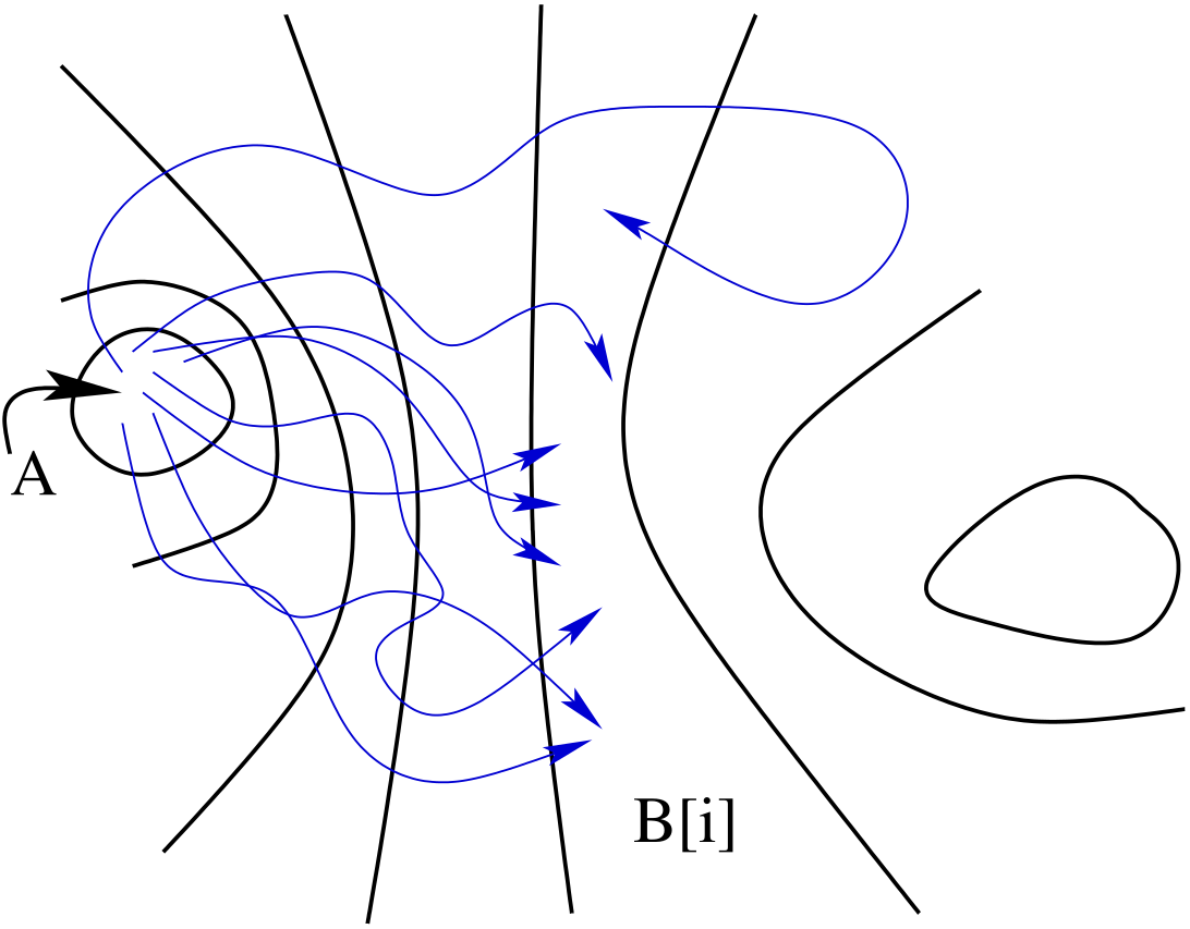
Let’s take stock: We know that \(k = dC/dt\). In order for \(k\) to be a constant, we need to ensure that \(C(t)\) is linear in time, meaning we must evaluate \(C(t)\) for many values of \(t\). Each evaluation of \(C(t)\) is a “free energy” calculation, so getting at \(k\) this way may be prohibitively expensive. Another insight of Dellago and Chandler [18] was to recognize that a simple factorization of \(C(t)\) leads to an algorithm in which one need only do a single free energy calculation. Consider: \begin{equation} C\left (t\right ) = \frac {\left \langle h_Ah_B\left (t\right )\right \rangle }{\left \langle h_Ah_B\left (t^\prime \right )\right \rangle } \times \frac {\left \langle h_Ah_B\left (t^\prime \right )\right \rangle }{h_A} = \frac {\left \langle h_Ah_B\left (t\right )\right \rangle }{\left \langle h_Ah_B\left (t^\prime \right )\right \rangle } \times C\left (t^\prime \right ), \end{equation} where both \(t\) and \(t^\prime \) are in an interval denoted \([0,T]\). For notational convenience: \(h_A\equiv h_A\left (x_0\right )\) and \(h_B(t)\equiv h_B\left (x_t\right )\).

Next, we define a new indicator function as a property of the interval \([0,T]\): \begin{equation} H_B\left (x_0,T\right ) \equiv \max _{0\le t\le T} h_B\left (x_t\right ) \end{equation} which tells us if the trajectory begun at \(x_0\) visits state \(B\) at least once during the interval \([0,T]\). Since \(H_B = 0\) if \(h_B(t) = 0\) for all \(t \in \left [0,T\right ]\), and \(H_B = 1\) otherwise, we can insert it into our factorized expression for \(C(t)\): \begin{equation}\label {eq:tps_9} C\left (t\right ) = \frac {\left \langle h_Ah_B\left (t\right )H_B\left (T\right )\right \rangle }{\left \langle h_AH_B\left (T\right )\right \rangle }\times \frac {\left \langle h_AH_B\left (T\right )\right \rangle }{\left \langle h_Ah_B\left (t^\prime \right )H_B\left (T\right )\right \rangle } \times C\left (t^\prime \right ), \end{equation} (We’ve also multiplied and divided by \(\left \langle h_AH_B\left (T\right )\right \rangle \).)

If we stare at Eq. 234 long enough, we see that the quantity \begin{equation} \begin {aligned} \left \langle h_B\left (t\right )\right \rangle _{AB} & \equiv \frac {\left \langle h_Ah_B\left (t\right )H_B\left (T\right )\right \rangle }{\left \langle h_AH_B\left (T\right )\right \rangle } \\ & = \frac {\int dx_0\rho \left (x_0\right )h_A\left (x_0\right )H_B\left (x_0,T\right )h_B\left (x_t\right )}{\int dx_0\rho \left (x_0\right )h_A\left (x_0\right )H_B\left (x_0,T\right )} \end {aligned} \end{equation} is an average of \(h_B(t)\) over the distribution function \begin{equation} F_{AB}\left (x_0,T\right ) \equiv \rho \left (x_0\right )h_A\left (x_0\right )H_B\left (x_0,T\right ) \end{equation} This is the ensemble of all paths that begin in \(A\) and visit \(B\) at least once in the interval \([0,T]\). (It therefore differs from \(f_{AB}\left (x_0,T\right )\).)

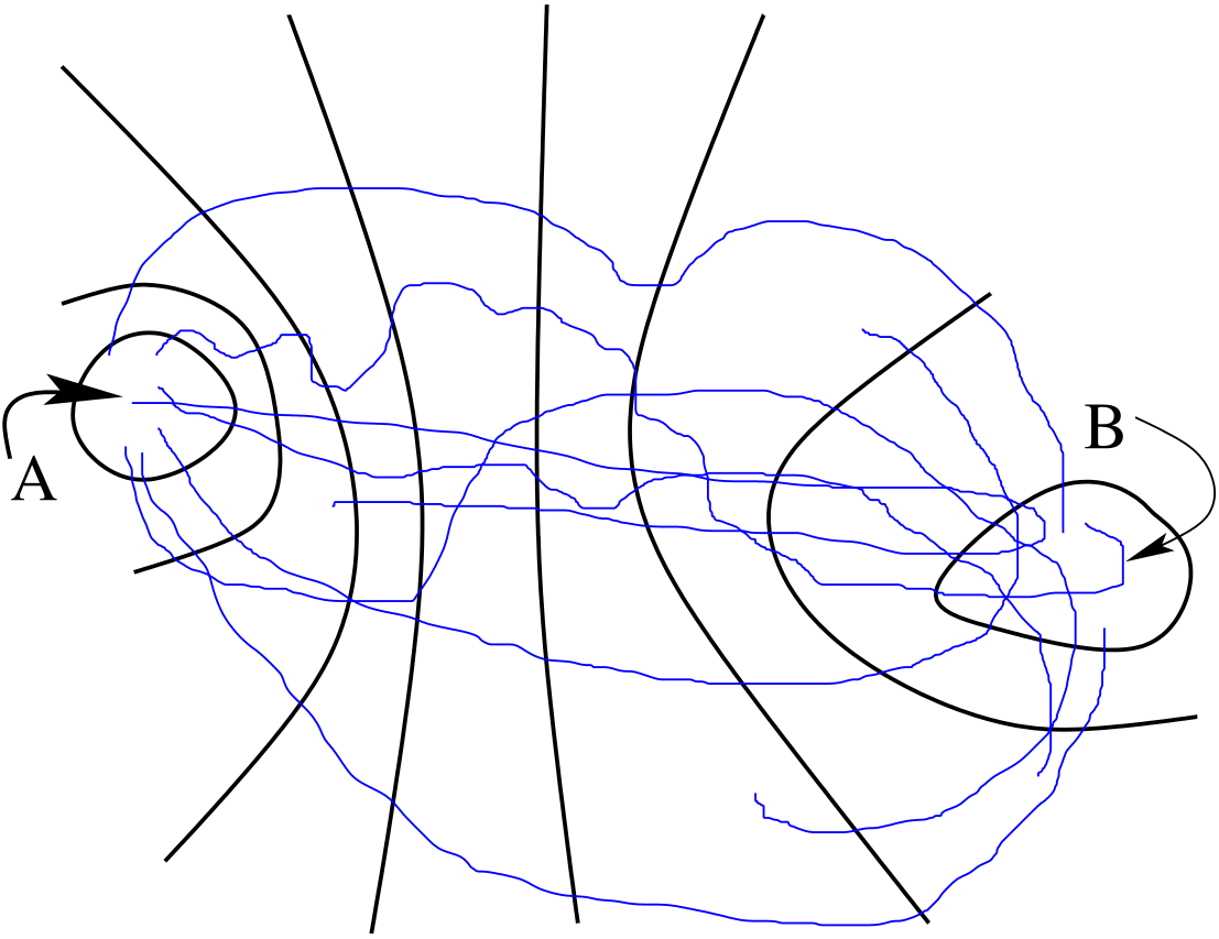
Using this notation to denote averaging over this ensemble, \(\left \langle \cdots \right \rangle _{AB}\), \begin{equation}\label {eq:tps_10} C\left (t\right ) = \frac {\left \langle h_B\left (t\right )\right \rangle _{AB}}{\left \langle h_B\left (t^\prime \right )\right \rangle _{AB}}C\left (t^\prime \right ) \end{equation} We can efficiently calculate \(\left \langle h_B\left (t\right )\right \rangle _{AB}\) by sampling \(F_{AB}\left (x_0,T\right )\) in a single simulation. \(C(t^\prime )\) can be calculated from a single free-energy umbrella-sampling calculation. This provides a recipe for obtaining \(k\):

1. Perform path sampling on \(F_{AB}\left (x_0,T\right )\) to obtain the function \(\left \langle h_B\left (t\right )\right \rangle _{AB}\) on \([0,T]\). If \(\frac {d}{dt}\left \langle h_B\left (t\right )\right \rangle _{AB}\) does not display a plateau, repeat with a larger value of \(T\).
2. Choose a time \(t^\prime \) (which can be much less than \(T\)) and compute \(P\left (\lambda ,t^\prime \right )\) by umbrella sampling to get \(C(t^\prime )\) by integration of Eq. 225. Because of step 1, \(\left \langle h_B\left (t^\prime \right )\right \rangle _{AB}\) is known.
3. Calculate \(C(t)\).
4. Calculate \(k(t)\) as \begin{equation} k\left (t\right ) = \frac {dC\left (t\right )}{dt} = \frac {\left \langle \dot {h}_B\left (t\right )\right \rangle _{AB}}{\left \langle h_B\left (t^\prime \right )\right \rangle _{AB}}\times C\left (t^\prime \right ) \end{equation}

7.2.3 Sampling the Transition Path Ensembles: Trial Moves

So, we see now that, using the factorization trick, we have two ensembles to average over: \[\begin {array}{rcl} f_{AB}\left (x_0,t\right ) & : & \text {distn. fcn. of all paths starting at } A \text { and ending in } B \text { at time } t \text {, used to compute } P\left (\lambda ,t\right )\\[4pt] F_{AB}\left (x_0,T\right ) & : & \text {distn. fcn. of all paths starting at } A \text { and visiting } B \text { at least once in the interval } [0,T] \text {, used to compute } \left \langle \dot {h}_B(t)\right \rangle _{AB} \text { and } \left \langle h_B(t^\prime )\right \rangle _{AB}. \end {array}\]

We can compute averages in these two ensembles by MC sampling. A new path is generated from an old path, and is accepted or rejected based on a detailed balance criterion. Now, we sample these two path ensembles in two different simulations, but the acceptance rules and trial moves are the same. Let’s generall call \(\mathscr {N}\left (i\right )\) the probability of path \(i\). We start with an old path “\(o\)” and attempt to generate a new path “\(n\)”. The acceptance rule obeying detailed balance is \begin{equation} \frac {{\rm acc}\left (o\rightarrow n\right )}{{\rm acc}\left (n\rightarrow o\right )} = \frac {\mathscr {N}\left (n\right )\alpha \left (n\rightarrow o\right )}{\mathscr {N}\left (o\right )\alpha \left (o\rightarrow n\right )} \end{equation}

\(\alpha \left (o\rightarrow n\right )\) is the a priori probabilit of attemptying to generate \(n\). The moves used in transition path sampling MC guarantee \(\alpha \left (o\rightarrow n\right ) = \alpha \left (n\rightarrow o\right )\). So,

So, what are the moves? There are two basic moves we can consider here.

• Given path \(o\), pick a configuration intermediate between \(A\) and \(B\), rotate all momenta by a little angle randomly selected from [-\(\Delta \phi \),\(\Delta \phi \)], and then MD integrate forwards and backwards to generate a new path. We accept if the backwards integration lands in A and the forwards in B. We get a high acceptance rate because \(A\) and \(B\) “attract” trajectories.
• Given path \(o\), chop off the first few \(\Delta t\)’s worth of its trajectory, and MD integrate from the end of another \(\Delta t\). If the beginning and end are still in \(A\) and \(B\) respectively, we accept the move. Note that this does not sample ergodically, but it does improve statistics over shooting alone. \(\Delta t\) can be positive or negative.

It seems the real trick is generating an initial path of length \(T\) that successfully connects region \(A\) with region \(B\). This can be done with traditional MD by beginning a trajectory in state \(A\) and simply waiting long enough for it to cross into \(B\). This might be possible, but could easily be prohibitively expensive. A better technique is to guess a path by creating a configuration which you hypothesize to be a transition state, and then integrating forward and backward in time to generate a path. It is accepted as an initial path if the beginning lands in \(A\) and the end in \(B\).

7.2.4 A Computational Model: Dimer Isomerization

To show the power of transition path sampling, it is perhaps best to consider a simple example of a two-state system where the states are separated by an energy barrier. This presentation is based on an exercise from the molecular simulation course taught by Berend Smit and Daan Frenkel in 2001, and uses a code called tps.

Here, we consider dimer isomerization in a simple 2D liquid sample of \(N\) 15 particles confined to a circle of radius \(R\). Particles 1 and 2 form the dimer. The total potential energy is given by \begin{equation} \mathscr {U} = {\sum _{i<j}}^\prime U_{\rm WCA}\left (r_{ij}\right ) + \sum _i U_{\rm wall}\left (r_i\right ) + U_{12}\left (r_{12}\right ) \end{equation} The prime indicates that the 1-2 pair is excluded from this sum. All particles interact with each other via a modified Lennard-Jones pairwise interaction known as the Weeks-Chandler-Andersen (WCA) potential: \begin{equation} U_{\rm WCA}\left (r\right ) = \left \{\begin {array}{ll} 4\left (r^{-12}-r^{-6}\right ) + 1 & \mbox {$r < 2^{1/6}$}\\ 0 & \mbox {$r > 2^{1/6}$} \end {array}\right . \end{equation} The WCA potential is fully repulsive, and cutoff where the force vanishes. The particles interact with the circular wall via another WCA potential: \begin{equation} U_{\rm wall}\left ({\bf r}\right ) = U_{\rm WCA}\left (R+2^{1/6}-r\right ) \end{equation} where \(\bf r\) is the vector position and \(r\) is the radial position (i.e., the circle is centered on the origin). The dimer bond (between particles 1 and 2) is described by a two-well potential: \begin{equation} U_{12}\left (r_{12}\right ) = h\left [1-\frac {\left (r_{12}-w-2^{1/6}\right )^2}{w^2}\right ]^2 \end{equation} This potential has stable minima at \(r_{12} = 2^{1/6}\) and \(r_{12} = 2^{1/6}+2w\). Here, \(h\) defines the height of the potential energy barrier between two stable states as defined by this potential, and \(w\) defines the width of this barrier:

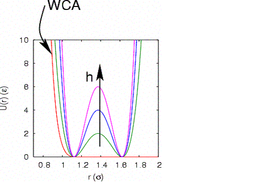
For now, we fix \(w\) at 0.25, and \(R\) at 3.0. This gives an areal particle number density \(\rho = 0.53~\sigma ^{-2}\).

What is a reasonable order parameter for this system? The bond length, naturally. All configurations for which \(r_{12} < 1.30\) are defined to be in region \(A\), and all configurations for which \(r_{12} > 1.45\) are defined be in region \(B\). It is important to note here that \(h\) is not a measure of the free energy barrier which determines the kinetic rate in this process. To determine the free energy barrier, we need to construct the free energy profile, \(F(r_{12}) = -k_BT\ln Q(r_{12})\). This type of restricted free energy is often termed a Landau free energy.

Let’s consider first a small potential barrier height, \(h = 2\). For this height, we can compute \(P(\lambda ,t\rightarrow \infty )\) very accurately from a single long MD simulation (10,000,000 steps; \(\Delta t\) = 0.001; total energy 15 \(\epsilon \)). We see from the linear region of \(C(t)\) that the rate constant appears to be \(k_{AB} = 4.04\times 10^{-2}~\tau ^{-1}\). Now, let us perform transition path sampling MC on this system.

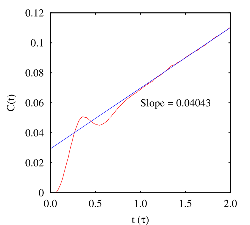
First, let’s decide how long an interval \(T\) we need. Clearly, \(C(t)\) appears to be linear up to \(t = 2\); following Dellago, we’ll choose \(T\) = 2.0. ⁴ Now, we need to conduct two types of MC simulations:

1. A single path sampling MC simulation to compute \(\left \langle \dot {h}_B(t)\right \rangle _{AB}\) and \(\left \langle h_B(t^\prime )\right \rangle _{AB}\) for \(0 < t,t^\prime < T\). We will conduct a simulation of \(10^6\) cycles.

2. A set of umbrella sampling MC simulations on the following intervals for \(r_{12}\):

   \(i\)	min	max
   1	0.00	1.22
   2	1.20	1.26
   3	1.24	1.30
   4	1.28	1.45
   5	1.40	2.45

   When matching the histograms in each of these intervals and renormalizing, we obtain \(P\left (r_{12},t=2\right )\). When we then integrate from \(r_{12} = 1.45\) to \(r_{12} = 2.45\) (region \(B\)).

We’ll use the other default parameter values provided in tps. These include the maximum angle by which velocity vectors are rotated in a shooting move (\(\Delta \phi = 0.6\) rad), and the number of shifting moves per shooting move (95:5), and the number of \(r_{12}\)-slices per window (200).

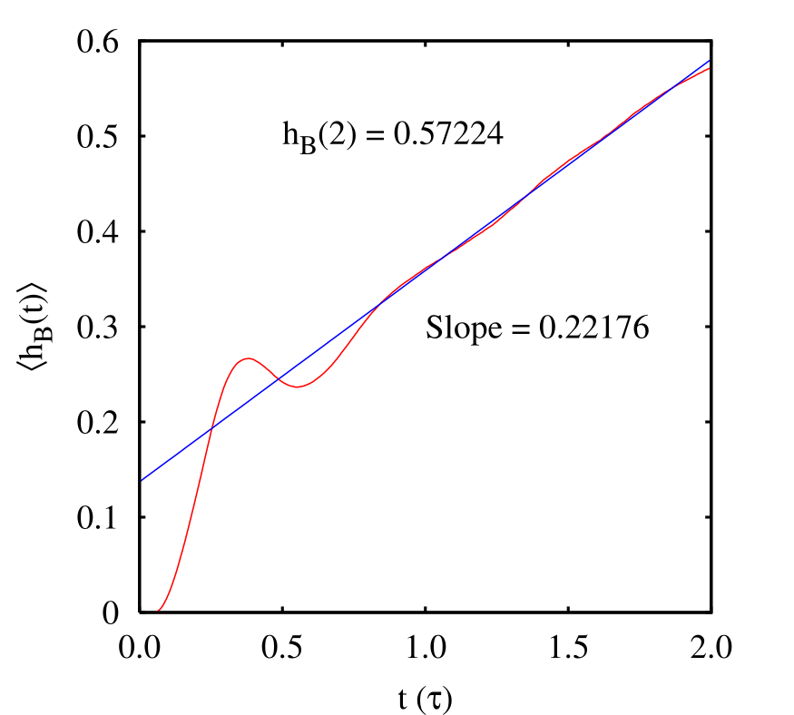
We see that \(\left \langle \dot {h}_B(t)\right \rangle = 0.22\) and \(\left \langle h_B(2)\right \rangle = 0.55\).

Now, the histogram:

We see that \(\left \langle \dot {h}_B(t)\right \rangle = 0.22\) and \(\left \langle h_B(2)\right \rangle = 0.55\).

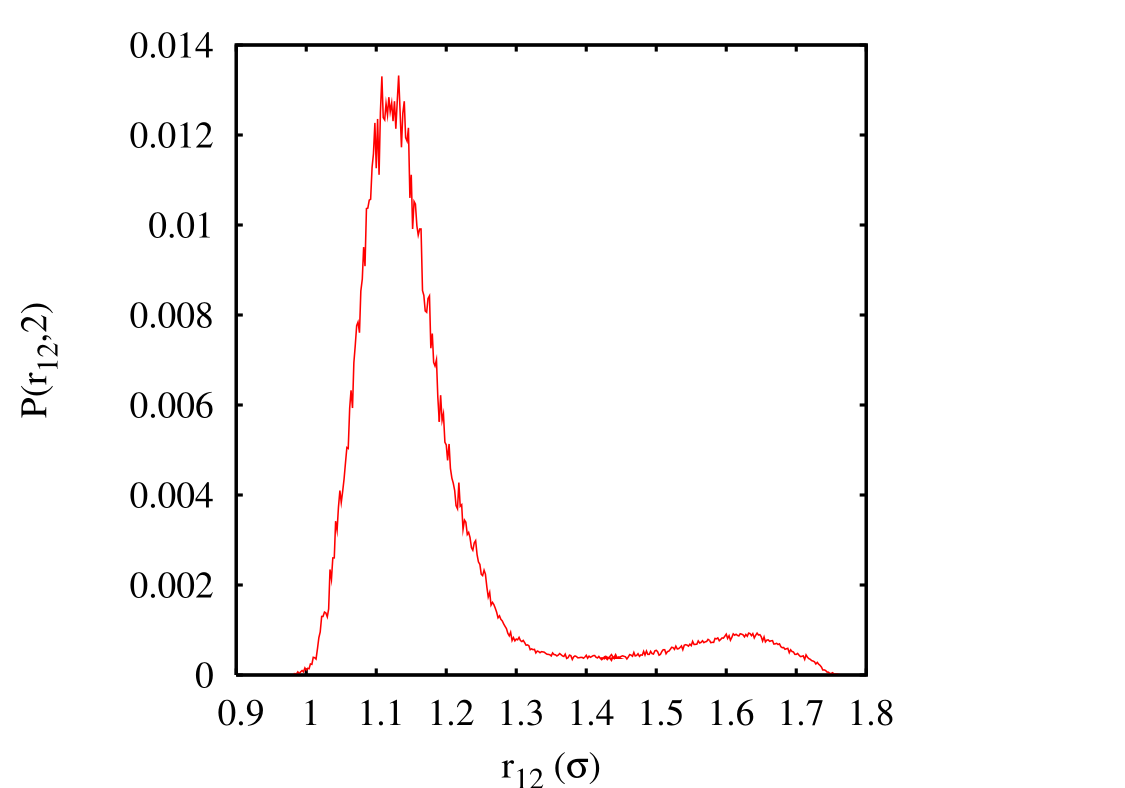
Integrating over region \(B\) yields \(C(2)\) = 0.09037. Performing the requisite operations yields \(k_{AB} = 0.0360~\tau ^{-1}\), which compares well to the MD-calculated value \(k_{AB} = 4.04\times 10^{-2}~\tau ^{-1}\).

Repeating this entire procedure for \(h\) = 6 yields \(k_{AB} = 5.05\times 10^{-4}~\tau ^{-1}\).

[to be completed; runs currently executing, June 30, 2026]