7.1 Case Study: Stillinger-Weber Silicon and the Tersoff Potential

No one should have the impression that people who do molecular simulation only care about the Lennard-Jones fluid. It has been and continues to be an important test-bed for theories of the liquid state and phase-equilibria. Nevertheless, molecular simulation has been performed on a wide variety of materials.

As a single example, consider silicon. Perhaps the earliest attempt to use molecular simulation to study a realistic atomic-scale model of silicon was due to Stillinger and Weber [16]. I “cut my teeth” on the Stillinger-Weber potential coding up my first real research code in graduate school. I now make a version of that code available to the students in this course, available at mdswsi.c. This code computes in reduced units as well; \(\sigma \) = 0.20951 nm, \(\epsilon \) = 2.1678 eV, and \(m\) = 28.085 amu, which are appropriate for a system of pure silicon. One reduced unit of temperature, \(T [=] \epsilon /k_B\), corresponds to 25156.73798 K.

The main reason to introduce Stillinger-Weber silicon here is to give you an example of a three-body potential. Silicon forms 4-coordinated tetrahedral bonded structures. The object of the three-body component of the potential is to enforce the tetrahedral bond angle (109.47\(^\circ \)) among triplets of bonded atoms.

The total potential is expressed as two sums, one for unique pair interactions, and another for unique triplet interactions:

The two-body models the bonds: \begin{equation} v_2 \left (r\right ) = \left \{\begin {array}{ll} \epsilon A \left (Br^{-p}-r^{-q}\right )\exp \left [\left (r-a\right )^{-1}\right ], & \mbox {$r < a$}\\ 0 & \mbox {$r\ge a$} \end {array} \right . \end{equation} It is very much like a Lennard-Jones potential, only with different exponents and a “smooth cutoff” as the interatom separation distance, \(r\), approaches some cutoff, \(a\), given by the factor \(\exp \left [\left (r-a\right )^{-1}\right ]\).

The three body models the angles, and is the sum of functions of each of the three angles of a triplet, \(ijk\):

Here I have employed the shorthand notation \(\displaystyle h_{jik} \equiv h\left (r_{ij}, r_{ik}, \theta _{jik}\right )\). Note that, in the notation of this potential, \(\theta _{jik}\) is subtended at \({\bf r}_i\), and \(\cos \theta _{jik}^c = -\frac {1}{3}\):

One computes the angle-\(j\) term, \(h_{ijk}\), and the angle-\(k\) term, \(h_{ikj}\), by permuting the indices appropriately.

The parameters used in the original study by Stillinger and Weber are: \begin{equation} \begin {aligned} A & = 7.049556277 \\ B & = 0.6022245584 \\ p & = 4 \\ q & = 0 \\ a & = 1.80 \\ \lambda & = 21.0 \\ \gamma & = 1.20 \end {aligned} \end{equation}

As in any MD simulation, one computes the force on any particle \(i\) from the negative gradient of the total potential: \begin{equation} \begin {aligned} {\bf f}_i & = -\nabla _{{\bf r}_i}\mathscr {U} \\ & = -\sum _{j\ne i} \nabla _{{\bf r}_i}v_2\left (r_{ij}\right ) - \sum _{j\ne i}\sum _{k\ne i,j} \nabla _{{\bf r}_i}v_3\left ({\bf r}_i,{\bf r}_j,{\bf r}_k\right ) \end {aligned} \end{equation}

The two-body term for the \(i\)-\(j\) interaction is only slightly more complicated than Lennard-Jones, due to the smooth cutoff. Here, assuming \(i\) and \(j\) are within interaction range (\(r_{ij} < a\)), we have for the force on \(i\) due to \(j\): \begin{equation}\label {eq:swfij} \begin {aligned} -\nabla _{{\bf r}_i} v_2\left (r_{ij}\right ) &= -\frac {\partial }{\partial {\bf r}_i} \left \{\epsilon A \left (Br_{ij}^{-p}-r_{ij}^{-q}\right )\exp \left [\left (r_{ij}-a\right )^{-1}\right ]\right \} \\ &= -\epsilon A \frac {{\bf r}_{ij}}{r_{ij}}\left (\left .\left [\frac {\partial }{\partial r} \left (Br^{-p}-r^{-q}\right )\right ]\right |_{r_{ij}}\exp \left [\left (r_{ij}-a\right )^{-1}\right ]\right . \\ &+ \left .\left (Br_{ij}^{-p}-r_{ij}^{-q}\right )\left .\left \{\frac {\partial }{\partial r}\exp \left [\left (r-a\right )^{-1}\right ]\right \}\right |_{r_{ij}}\right ) \\ &= -\epsilon A \frac {{\bf r}_{ij}}{r_{ij}}\left \{\left (-pBr_{ij}^{-p-1}+qr_{ij}^{-q-1}\right )\exp \left [\left (r_{ij}-a\right )^{-1}\right ]\right . \\ &- \left .\left (Br_{ij}^{-p}-r_{ij}^{-q}\right )\exp \left [\left (r_{ij}-a\right )^{-1}\right ]\left (r_{ij}-a\right )^{-2}\right \} \\ &= v_2\frac {{\bf r}_{ij}}{r_{ij}}\left [\frac {pBr_{ij}^{-p-1}-qr_{ij}^{-q-1}}{Br_{ij}^{-p}-r_{ij}^{-q}} + \left (r_{ij}-a\right )^{-2}\right ] \\ &\equiv {\bf f}_{ij} \end {aligned} \end{equation} Note that it is still true that \({\bf f}_{ij} = -{\bf f}_{ji}\). Exercise: Show that the right-hand-side of Eq. 185 is well-behaved (that is, it does not diverge, and in fact vanishes) as \(r_{ij}\rightarrow a^-\).

It is comparatively much more tedious to evaluate the three-body gradients. \begin{equation}\label {eq:sw3_partials} \begin {aligned} -\nabla _{{\bf r}_i}v_3\left ({\bf r}_i,{\bf r}_j,{\bf r}_k\right ) &= -\nabla _{{\bf r}_i}\left (h_{jik} + h_{ijk} + h_{ikj}\right ) \\ &= -\left (\frac {\partial h_{jik}}{\partial {\bf r}_i} +\frac {\partial h_{ijk}}{\partial {\bf r}_i} +\frac {\partial h_{ikj}}{\partial {\bf r}_i}\right ) \\ &\equiv {\bf f}_{i\leftarrow jk} \end {aligned} \end{equation} The triplet forces on the other members of the triplet, \({\bf f}_{j\leftarrow ik}\) and \({\bf f}_{k\leftarrow ij}\), are defined analogously.

Each of the partials in Eq. 186 is unique: \begin{equation} \label {eq:sw3jik} \begin {array}{lll} \mbox {\raisebox {-0.5cm}{\includegraphics [width=1cm]{figpng/hjik.png}}\ \ } \displaystyle {\frac {\partial h_{jik}}{\partial {\bf r}_i}} & \displaystyle = &\displaystyle - \gamma h_{jik}\left [ {{{\bf r}_{ij}}\over {r_{ij}}}{{1}\over {\left (r_{ij}-a\right )^2}} + \frac {{\bf r}_{ik}}{r_{ik}}\frac {1}{\left (r_{ik}-a\right )^2} \right ] \\ & \displaystyle + & \displaystyle 2\lambda \exp \left ( \frac {\gamma }{r_{ij}-a} + \frac {\gamma }{r_{ik}-a} \right ) \left (\cos \theta _{jik}-\cos \theta _{jik}^c\right ) \\ & \displaystyle \times & \displaystyle \left [ \frac {{\bf r}_{ij}}{r_{ij}}\frac {1}{r_{ik}} +\frac {{\bf r}_{ik}}{r_{ik}}\frac {1}{r_{ij}} -\left (\frac {{\bf r}_{ij}}{r_{ij}}\frac {1}{r_{ik}} +\frac {{\bf r}_{ik}}{r_{ik}}\frac {1}{r_{ij}}\right ) \cos \theta _{jik}\right ] \end {array} \end{equation} \begin{equation} \label {eq:sw3ijk} \begin {array}{lll} \mbox {\raisebox {-0.5cm}{\includegraphics [width=1cm]{figpng/hijk.png}}\ \ } \displaystyle \frac {\partial h_{ijk}}{\partial {\bf r}_i} & \displaystyle = & \displaystyle - \gamma _j h_{ijk}\left [ \frac {{\bf r}_{ij}}{r_{ij}}\frac {1}{\left (r_{ij}-a\right )^2} \right ] \\ & \displaystyle + & \displaystyle 2\lambda _j\exp \left ( \frac {\gamma _j}{r_{ij}-a} + \frac {\gamma _j}{r_{jk}-a} \right ) \left (\cos \theta _{ijk}-\cos \theta _{ijk}^c\right ) \\ & \displaystyle \times & \displaystyle \left [ \frac {{\bf r}_{jk}}{r_{jk}}\frac {1}{r_{ij}} +\frac {{\bf r}_{ij}}{r_{ij}}\frac {1}{r_{ij}} \cos \theta _{ijk}\right ] \end {array} \end{equation} \begin{equation} \label {eq:sw3ikj} \begin {array}{lll} \mbox {\raisebox {-0.5cm}{\includegraphics [width=1cm]{figpng/hikj.png}}\ \ } \displaystyle \frac {\partial h_{ikj}}{\partial {\bf r}_i} & \displaystyle = & - \displaystyle \gamma _k h_{ikj}\left [ \frac {{\bf r}_{ik}}{r_{ik}}\frac {1}{\left (r_{ik}-a\right )^2} \right ] \\ & \displaystyle + & \displaystyle 2\lambda _k\exp \left ( \frac {\gamma _k}{r_{ik}-a} + \frac {\gamma _k}{r_{jk}-a} \right ) \left (\cos \theta _{ikj}-\cos \theta _{ikj}^c\right ) \\ & \displaystyle \times & \displaystyle \left [ -\frac {{\bf r}_{jk}}{r_{jk}}\frac {1}{r_{ik}} +\frac {{\bf r}_{ik}}{r_{ik}}\frac {1}{r_{ik}} \cos \theta _{ikj}\right ] \end {array} \end{equation} Note that the right hand sides of each of Eqns. 187, 188, and 189 vanish when the appropriate \(r\)’s are greater than \(a\)’s, as in Eq. 212. Exercise: Show that \({\bf f}_{i\leftarrow jk} + {\bf f}_{j\leftarrow ik} + {\bf f}_{k\leftarrow ij} = 0\).

We can investigate what happens when we willfully ignore the three-body terms. Let us initialize atoms on a diamond-cubic lattice (the minimal energy lattice of silicon); a snapshot appears below.

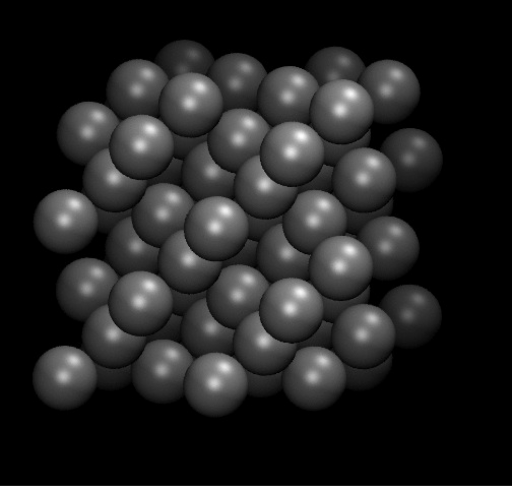
Let us now run two MD simulations for 10,000 time steps; one with and and the other without three body forces, at reduced initial temperature \(T\) = 0.12 and reduced density \(\rho \) = 0.46 for a small system of 64 atoms. You can download small 64-atom system configuration here, already equilibrated at \(T\)=0.12 (pictured above). Note that you must compile the code mdswsi.c with the flag -DTHREEBODY to include three-body forces. You can create an executable version of mdswsi that ignores three-body forces by compiling without the flag -DTHREEBODY. For example:

% gcc -o mdswsi_no3 mdswsi.c -lm -lgsl
% gcc -o mdswsi mdswsi.c -DTHREEBODY -lm -lgsl

Note also that this code uses the Andersen thermostat by default, with a default value of \(\nu \) = 0.1. This can be overridden (or turned off) by specifying a value of \(\nu \) on the command line. For example,

% mdswsi -nu 0 -ns 10001 -icf init.xyz

turns off the thermostat, which is what I have done for this little demonstration.

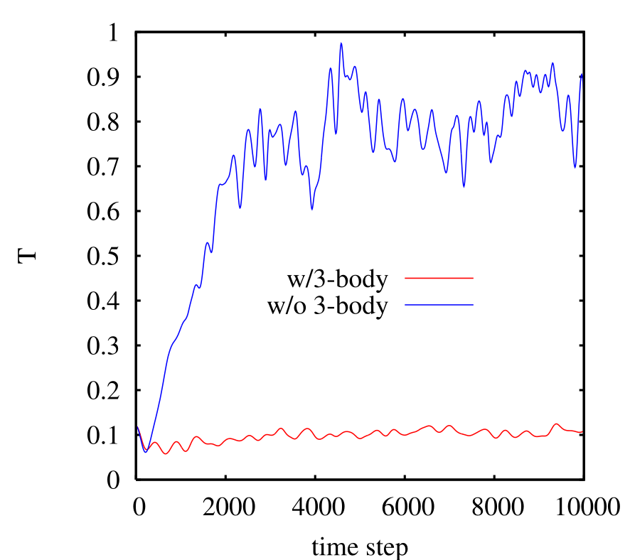
Below we plot the instantaneous temperature vs. time-step (0.001 \(\tau \)) for the two runs. Notice that the system with the 3-body forces intact remains steady at \(T \approx \) 0.12, while the system without 3-body forces simply “melts,” with \(T\) approaching 20,000 K A quick look at a configuration (not shown) reveals that there is no longer any crystalline order; the system is now an amorphous blob of silicon atoms. The lesson of this little demonstration is that one must have three-body forces to stabilize a diamond-cubic lattice.

As a suggested project, you can try one or more of several things with this code.

1. The force routine involves a triplet loop, which is extremely costly. Were one to double the size of the system, the computational effort would increase by a factor of eight. Appendix F in F&S discusses algorithms to speed up force evaluation by taking advantage of finite interaction ranges. Can you make the triplet loop more efficient using these techniques? (My thesis code used a unique version of the Verlet List technique.)
2. Use the code rdf.c to compute the radial distribution function of both crystalline and liquid silicon. Can you explain the differences between these two, and from the \(g(r)\) for a simple LJ liquid?
3. Can you compute the diffusivity of a Si atom in a liquid?