4.2 Case Study 1: The 2D Ising Magnet
4.2.1 Introduction
In the introductory lecture, I introduced state-counting using a simple, one-dimensional Ising system. To be precise, this was a particular case known as an Ising magnet of noninteracting spins, because each spin made its own independent contribution to the Hamiltonian. The state of the magnet is specified by specifying each spin variable as either +1 or -1:
Now, we will consider a more interesting Ising system; namely, that of interacting spins on a 2d square lattice. What do we mean by interacting? We mean that the Hamiltonian depends on pairs of spins: \begin{equation} \label {eq:2dising} \mathscr {H} = -J\sum _{\left <ij\right >}s_is_j \end{equation} where the notation \(\left <ij\right >\) denotes that we are summing over unique pairs of nearest neighbors, and, as before a spin \(s_i\) is either +1 or -1. \(J\) is the “coupling constant” and represents our default unit of energy. How many unique pairs of nearest neighbors are there on a lattice of \(N\) spins (assuming periodic boundary conditions)? To answer this question, we must know the coordination, \(z\), of the lattice; that is, how many nearest neighbors does one lattice position have? For a square lattice, \(z\) = 4. Each spin therefore contributes two unique spin pairs to the system, so there are \(Nz/2\) unique nearest neighbor pairs.
Think about this Hamiltonian. It says that energy is minimal when all \(N\) spins have the same alignment, either all up or all down. Imagine a microscopic observable called the magnetization, or average spin orientation, \(M\): \begin{equation} M \equiv \frac {1}{N} \sum _i^N s_i \end{equation} Then, \(M\) = +1 and -1 are two energetically equivalent microstates. We can then expect that if there is any thermal energy in the system which randomly flips spins, the amount of this thermal energy (that is, the temerature) will somehow control the observable magnetization. We “observe” magnetization using an ensemble average: \begin{equation} \label {eq:magnetization} \left <M\right > = \frac {\displaystyle \sum _{s_1=-1}^{+1} \cdots \sum _{s_N=-1}^{+1} \left [\sum _i^N s_i\right ]\exp \left [-\beta \mathscr {H}\left (s_1,\dots ,s_N\right )\right ]} {\displaystyle \sum _{s_1=-1}^{+1} \cdots \sum _{s_N=-1}^{+1} \exp \left [-\beta \mathscr {H}\left (s_1,\dots ,s_N\right )\right ]} \end{equation} Our physical intuition tells us that as \(T\rightarrow \) 0, \(\left |\left <M\right >\right |\rightarrow \) 1, and as \(T\rightarrow \infty \), \(\left <M\right >\rightarrow \) 0. The fascinating thing about an Ising magnet is that there is a finite temperature called the critical temperature, \(T_c\). If we start out with a “hot” system, and cool it to just below \(T_c\), the absolute value of the magnetization spontaneously jumps from 0 to some finite value. In other words, the system undergoes a phase transition from a disordered phase to a partially ordered phase. A Metropolis Monte Carlo simulation can allow us to probe the behavior of an Ising system and learn how the system behaves near criticality. The rest of this case study will be devoted to showing you the inner workings of a C program which simulates the Ising magnet using Metropolis MC, as a first implementation of this technique. In the suggested exercises appearing at the end of this case study, you will modify this code slightly to compute averages values of certain observables.
But first, I recommend you check out this Java implementation of a Monte Carlo simulation of a 2-dimensional Ising magnet (one of many on the web; google “ising simulation” and you’ll get a nice sample.) This is a fun little Java applet that lets you play with an Ising magnet. You can change the temperature of the simulation: making it cold will “freeze” the system, and making it hot “melts” it. Near the critical temperature, \(T_c\), relatively large regions of mostly-up spins compete with regions of mostly down spin. In one of the exercises, we’ll learn how to measure an observable called the correlation length, which characterizes the size of these domains and is a useful signature of criticality.
4.2.2 A C Code for the 2D Ising Magnet
In this section, we will dissect piece-by-piece a small C program that implements an NVT Metropolis Monte Carlo simulation of a 2D Ising magnet.
If you have not already done so, clone the Abrams-Teaching/instructional-codes repository from Github.
This repository will be updated throughout the term with source code in the originals subdirectory. You
should create a subdirectory called my_work inside this repository and do all editing, compiling, and running in
there. This directory is specifically excluded from git revision control by its inclusion in the .gitignore
file. This way, when I put new codes in the repository, you only have to git pull to download
them.
cd
cd cheT580
git clone git@github.com:Abrams-Teaching/instructional-codes.git
cd instructional-codes
mkdir my_work
cd my_work
cp ../originals/ising_mc.c .
code .
From a terminal command-line inside VSCode, or outside, you can compile ising_mc.c via
gcc -O3 -o ising ising_mc.c -lm -lgsl
and you can then run it at the command line as ./ising. It has a lot of options for controlling the size
of the magnet (the number of spins), the temperature, and other parameters, which I’ll go over
now.
ising_mc.c conducts a canoncial Metropolis Monte Carlo simulation of an Ising magnet of size \(L\times L\) at
temperature \(T\) (both specified by the user at run time on the command line), and it computes both the average
energy per spin \(\left <\epsilon \right >\) and the average spin value, \(\left <s_1\right >\).
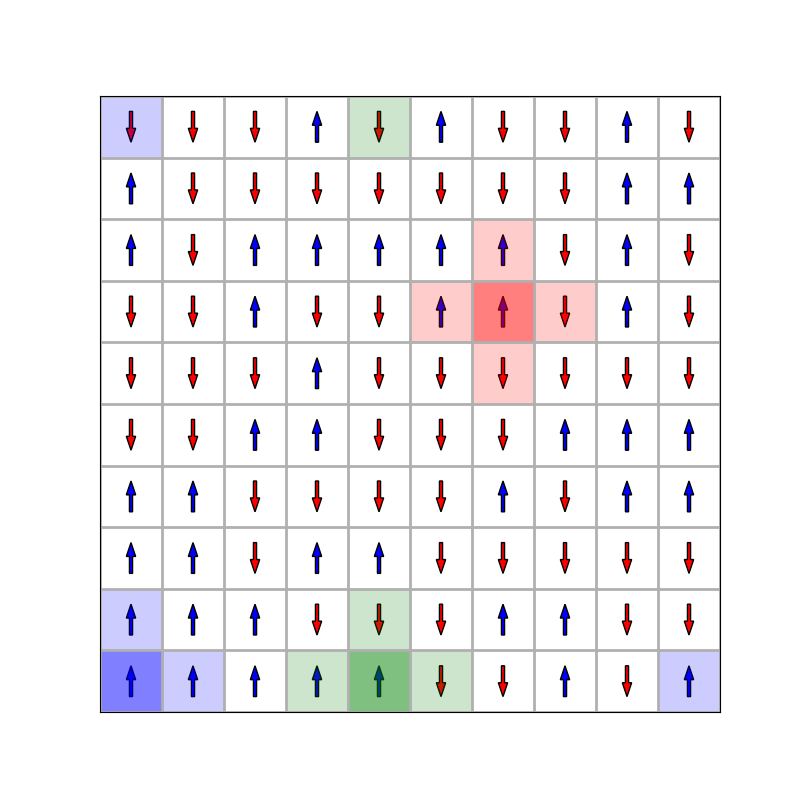
Periodic boundaries are employed in calculating the nearest-neighbor interactions. Consider an \(L\times L\) magnet; each row \(i\) indexed from 0 to \(N-1\) has \(L\) columns also indexed from 0 to \(N-1\). If the cell at (5,5) queries its neighbors, they are at (4,5), (6,5), (5,4), and (5,6). However, the cell at (0,5) would have a southern neighbor at (\(N-1\),5) instead of (-1,5), since there is no row indexed -1! Fig. 3 demonstrates this.
An abbreviated listing of the code follows. Some comments in the full, downloadable code have been omitted for space, and I have instead explained each code fragment in accompanying text.
Headers
These are some standard headers we include in most C programs, along with the GNU scientific library.
#include <stdio.h>
#include <stdlib.h>
#include <math.h>
#include <gsl/gsl_rng.h>
The Change in Energy upon a Proposed Spin Flip
dE() is function that accepts as arguments the 2D array of spins, M; the side-length, L, and a position \((i,j)\), and
returns the change in energy (in units of \(J\)) upon flipping spin \((i,j)\), without actually flipping it. All variables are of
integer type, int. The syntax ** M means that M is a pointer to a pointer to an int, signifying that M is a 2D
array. To access element in row i and column j in M, the syntax is M[i][j]. In C, all array indices start at 0, so
M[0][0] refers to the “upper-left” corner of the magnet (assuming row numbers increase going down the
magnet). The inline conditional syntax i?(i-1):(L-1) expands as, “If i is non-zero, return i-1; otherwise,
return L-1.” This implements periodic boundaries when looking to the west of spin M[i][j]. The syntax
(i+1)\%L returns computes \((i+1)\mod L\), which also implements periodic boundaries when looking to the east of spin
M[i][j].
int dE ( int ** M, int L, int i, int j ) {
  return -2*(M[i][j])*(M[i?(i-1):(L-1)][j]+M[(i+1)%L][j]+
        M[i][j?(j-1):(L-1)]+M[i][(j+1)%L]);
}
Initialize all Spin Values
The function init() visits every spin and assigns it either +1 or -1 randomly.
void init ( int ** M, int L, gsl_rng * r ) {
  int i,j;
  for (i=0;i<L;i++) {
    for (j=0;j<L;j++) {
      M[i][j]=2*(int)gsl_rng_uniform_int(r,2)-1;
    }
  }
}
Main Program: Variable Declarations
In C functions, including main(), all variables must be declared by type before they are used. Often, it makes
sense to initialize them to some default values upon declaration. Here, we make the default magnet 20\(\times \)20 in
size, set the temperature to 1 (in dimensions of \(J/k_B\)), and provide some defaults fo the number of cycles (10\(^6\)) and
sampling interval (10\(^3\)) in cycles (a cycle is one round of \(N\) attempted flips). Variables for holding a
couple of observables are initialized. Finally, the pseudorandom number generator from the GSL is
declared.
  int main (int argc, char * argv[]) {
  /* System parameters */
  int ** M;       /* The 2D array of spins */
  int L = 20;     /* The sidelength of the array */
  int N;          /* The total number of spins = L*L */
  double T = 1.0; /* Dimensionless temperature = (T*k)/J */

  /* Run parameters */
  int nCycles = 1000000; /* number of MC cycles to run;
                            one cycle is N consecutive attempted
                            spin flips */
  int fSamp = 1000;      /* Interval between taking samples */

  /* Computational variables */
  int nSamp;      /* Number of samples taken */
  int de;         /* energy change due to flipping a spin */
  double b;       /* Boltzman factor */
  double x;       /* random number */
  int i,j,a,c;    /* loop counters */

  /* Observables */
  double s=0.0, ssum=0.0;    /* average magnetization */
  double e=0.0, esum=0.0;    /* average energy per spin */

  /* Pseudorandom Number Generator */
  gsl_rng * r = gsl_rng_alloc(gsl_rng_mt19937);
  unsigned long int Seed = 23410981;
Main Program: Argument Parsing
Here, we parse the command line arguments. The user running the program can specify the magnet
side-length \(L\), the temperature (in units of \(J/k_B\)), the number of cycles, the sampling interval, and the seed value for
the pseudorandom number generator. The array argv[] and its count of elements argc appear as parameters
in the definition of main, as is customary in C. The built-in function strcmp() returns 0 if the two
arguments match, so the logical expression strcmp(a,b)! evaluates to TRUE if strings a and b
match. The built-in functions atoi() and atof() convert their string arguments to integers and
floating-points, respectively. The notation argv[++i] means that first the current value of i is
incremented by 1 and then it is used to access the value in argv[]. So, for example, if the string "-L"
is detected at the ith position in the array of command-line arguments, the code immediately
jumps to the next position in the array and tries to intepret that argument as an integer to assign to
L.
  for (i=1;i<argc;i++) {
    if (!strcmp(argv[i],"-L")) L=atoi(argv[++i]);
    else if (!strcmp(argv[i],"-T")) T=atof(argv[++i]);
    else if (!strcmp(argv[i],"-nc")) nCycles = atoi(argv[++i]);
    else if (!strcmp(argv[i],"-fs")) fSamp = atoi(argv[++i]);
    else if (!strcmp(argv[i],"-s")) {
      Seed = (unsigned long)atoi(argv[++i]);
    }
  }
Main Program: Initial Outputs
Next, we echo the command entered back to the terminal, and then output any parsed variables values.
  printf("# command: ");
  for (i=0;i<argc;i++) printf("%s ",argv[i]);
  printf("\n");
  printf("# ISING simulation, NVT Metropolis Monte Carlo\n");
  printf("# L = %i, T = %.3lf, nCycles %i, fSamp %i, Seed %lu\n",
   L,T,nCycles,fSamp,Seed);
Main Program: Initialization
Next, we initialize the pseudorandom number generator r by setting the seed value using Seed.
Then the number of spins \(N\) is computed assuming a square magnet. We then allocate memory
needed to hold the magnet; this is a standard method of allocating a 2D array of integers. Next
we call our init() function, and finally we convert \(T\) to \(1/T\) since multiplication is more efficient than
division.
  /* Seed the random number generator */
  gsl_rng_set(r,Seed);

  /* Compute the number of spins */
  N=L*L;

  /* Allocate memory for the system */
  M=(int**)malloc(L*sizeof(int*));
  for (i=0;i<L;i++) M[i]=(int*)malloc(L*sizeof(int));

  /* Generate an initial state */
  init(M,L,r);

  /* For computational efficiency, convert T to reciprocal T */
  T=1.0/T;
Main Program: Monte Carlo Loop
And now the loop. Note the outer loop counts cycles, and the inner loops counts flip attempts in one cycle. The
variables i and j are randomly assigned between 0 and \(L\)-1, identifying a random spin. This random
spin is tagged and sent to our dE() function to calculate the change in energy we would expect if
that spin were flipped (+1\(\rightarrow \)-1 or -1\(\rightarrow \)+1). We then calculate the Boltzmann factor in b, and then use
the Metropolis criterion to decide whether to accept or reject this spin flip: choosing a random
variable on [0,1] and accepting the move if the Boltzmann factor is greater than this number. If it is
accepted, we actually peform the flip by multiplying the spin value by -1. Finally, if the current
cycle is one in which we collect a sample, we do so by calling the samp() function. The logical
expression (c%fSamp)! evaluates to TRUE if the cycle counter c is divisible by fSamp. In the call
to samp(), the arguments s and e are passed by reference, signified by the & qualifier. This is
necessary because inside samp() we modify both variables. Each of s and e are added to their
respective tallies, ssum and esum, and the number of samples taken nSamp is incremented by
1.
  s = 0.0;
  e = 0.0;
  nSamp = 0;
  for (c=0;c<nCycles;c++) {
    /* Make N flip attempts */
    for (a=0;a<N;a++) {
      /* randomly select a spin */
      i=(int)gsl_rng_uniform_int(r,L);
      j=(int)gsl_rng_uniform_int(r,L);
      /* get the "new" energy as the incremental change due
         to flipping spin (i,j) */
      de = dE(M,L,i,j);
      /* compute the Boltzmann factor; recall T is now
         reciprocal temperature */
      b = exp(de*T);
      /* pick a random number between 0 and 1 */
      x = gsl_rng_uniform(r);
      /* accept or reject this flip */
      if (x<b) { /* accept */
       /* flip it */
       M[i][j]*=-1;
      }
    }
    /* Sample and accumulate averages */
    if (!(c%fSamp)) {
      samp(M,L,&s,&e);
      fprintf(stdout,"%i %.5le %.5le\n",c,s,e);
      fflush(stdout);
      ssum+=s;
      esum+=e;
      nSamp++;
    }
  }
Main Program: Final Outputs and Program Termination
After the outer loop finishes, we can finish up by reporting the averages \(\left <s_1\right >\) from the tallies of s and
e.
  fprintf(stdout,"# The average magnetization is %.5lf\n",
                 ssum/nSamp);
  fprintf(stdout,"# The average energy per spin is %.5lf\n",
                 esum/nSamp);
  fprintf(stdout,"# Program ends.\n");
}
4.2.3 Example: Average Energy and Magnetization vs. Temperature
Let’s run the code for an \(L\)=40 lattice for the following values of temperature: 5.0, 4.0, 3.0, 2.0, 1.0. At each temperature, we’ll run six separate simulations with a unique random number generator seed. Fig. 4 shows the average magnetization \(\langle s_1\rangle \) and the average energy per spin \(\langle e\rangle \) vs. temperature, with each simulation contributing a unique point.
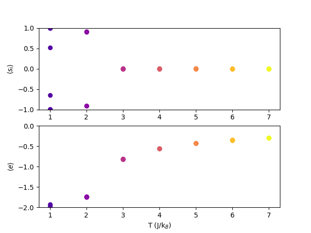
What is happening here? Clearly, as the temperature decreases, the average energy per spin approaches -2; this makes sense because the spins will tend to align with their neighbors. However, when we look at the average magnetization, we see that \(\langle s_1\rangle \) is zero at high temperatures but then can seemingly approach either +1 or -1 as the temperature goes down. This is because of symmetry breaking: although either all-up or all-down is equally likely, once it falls toward one it won’t ever climb back out and go to the other. So we see some magnets go to all -1 and others to all +1.
Symmetry-breaking is an important phenomenon in molecular simulations. The impact is has is to prevent exploration of state space because of barriers that are only extremely rarely overcome when resolving state-to-state transitions microscopically. In the low-\(T\) Ising magnet, the all-up and all-down states are equally likely, but once one is committed to, the other will never practically be explored. Why is this significant? Many systems have state spaces like this, where there are two or more high-probability regions separated by large regions of low probability. Sampling based on local moves in state space can almost never overcome such barriers, meaning such simulations are likely never truly ergodic. None of the MC simulations below about \(T\) = 2.2 for an Ising simulation are ergodic!
4.2.4 Suggested Exercises
- 1.
- Modify the code so that when samples are taken in accumulating statistics for \(\left <s_1\right >\) and \(\left <\epsilon \right >\), the current sample values are output to the terminal. You’ll want to find the right place to add the following line: fprintf(stdout,"%i %.5lf %.5lf\(\backslash \)n",c,s,e);
- 2.
- The current version of the code initializes the Ising lattice with random spins. What temperature does this correspond to? Modify the code so that the initial lattice has two well-defined domains, all spin-up for \(i < L/2\) and all spin-down for \(i > L/2\). Re-run at the various temperatures. Do you see any differences?
- 3.
- (Advanced) Modify the code ising.c to compute the quantity \(\left <s_is_j\right > - \left <s_i\right >\left <s_j\right >\) as a function of various distances between spins \(i\) and \(j\).