6.1 Monte Carlo Simulations in the Isothermal-Isobaric and Grand Canonical Ensembles
6.1.1 Isothermal-Isobaric
In this section, we consider how to conduct Monte Carlo simulation in ensembles other than the canonical ensemble. In deriving the partition function for the canonical ensemble (Eq. 38), we imagined our sytem of constant \(N\), \(V\), and \(T\) in thermal contact with a large reservoir. This thermal contact allowed the system and reservoir to exchange energy such that the system remained at constant \(T\), and what resulted was the Boltzmann factor. In Section 5.4.1, F&S explain the case when we have the reservoir and the system both thermally and mechanically coupled. The mechanical coupling allows the volume of the system to change such that the pressure in the system is the same as the reservoir, which is again considered as an inifinite ideal gas. In addition to thermostatting our system, the reservoir acts as a barostat.
First, for convenience, we express the set of coordinates, \({\bf r}^N\), scaled by the box length, \(L\), as \({\bf s}^N\). The partition function in the NPT ensemble is then \begin{equation} Q\left (N,P,T\right ) = \frac {\beta P}{\Lambda ^{3N}N!} \int dV V^N \exp \left (-\beta PV\right ) \int d{\bf s}^N \exp \left [-\beta \mathscr {U}\left ({\bf s}^N;L\right )\right ] \end{equation} The free energy associated with this ensemble is the Gibbs free energy: \begin{equation} G = -k_BT\ln Q\left (N,P,T\right ) \end{equation}
Now, compared to the canonical ensemble, in the NPT ensemble, volume is an additional degree of freedom. We need the probability distribution to include volume: \begin{equation} \begin {aligned} \mathscr {N}\left (V;{\bf s}^N\right ) & \propto V^N\exp \left (-\beta PV\right )\exp \left [-\beta \mathscr {U}\left ({\bf s}^N;L\right )\right ] \\ & = \exp \left \{-\beta \left [\mathscr {U}\left ({\bf s}^N,V\right ) + PV - N\beta ^{-1}\ln V\right ]\right \} \end {aligned} \end{equation} We can use this new Boltzmann factor in an acceptance rule for a Monte Carlo trial move involving a simple volume change from \(V\) to \(V + \Delta V\), where \(\Delta V\) is randomly chosen from \([-\Delta V_{max},\Delta V_{max}]\): \begin{equation} \mbox {acc}\left (o\rightarrow n\right ) = \min \left (1,\exp \left \{ -\beta \left [\mathscr {U}\left ({\bf s}^N,V^\prime \right )-\mathscr {U}\left ({\bf s}^N,V\right )+P\left (V-V^\prime \right )-N\beta ^{-1}\ln \left (V^\prime /V\right )\right ]\right \}\right ) \end{equation}
We can also consider trial move that changes the logarithm of the box size from \(\ln V\) to \(\ln V + \Delta \left (\ln V\right )\). In this case, the integral of \(V^N\) over \(dV\) is re-expressed as an integral of \(V^{N+1}\) over \(d\ln V\), and the acceptance rule is the same as the one above except for a factor of \((N+1)\) multiplying \(\beta ^{-1}\), instead of \(N\).
The C-code mclj_npt.c implements an NPT MC simulation of the Lennard-Jones liquid using both particle
displacements and log-\(V\) displacements. For each cycle, there is a \(1/(N+1)\) probability that a trial move is a volume
displacement. The trial move generates a random displacement, computes a new box length, rescales all
particle positions, scales the cutoff radius, and recomputes the tail corrections and shift, if applicable. If the
Metropolis criterion is not met after a random number is selected, then all of these operations are undone.
Otherwise, the new box size with the newly scaled particle positions is kept. The particle displacement
algorithm is the same as in mclj.c.
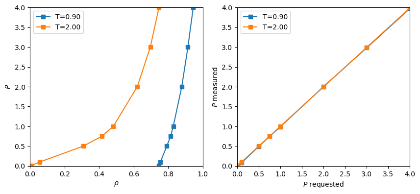
As an exercise, you can use the code to regenerate Figure 5.3 in the text, which is again a slice through the phase diagram of the Lennard-Jones fluid at \(T\) = 2.0. This temperature is above the critical tempeerature, so we do not anticipate a phase transition at the pressures investigated. However, we saw that when we considered \(T\) = 0.9 using the NVT MC simulation, negative pressures were predicted, indicating that the system would have liked to phase separate but couldn’t due to its fixed density and finite size. That is, at the density specified, there might not be enough particles to “nucleate” the denser of the two phases. NPT simulations in principle offer a way around that by allowing the system density to fluctuate.
I ran the code with \(N\) = 108 particles for 10\(^6\) cycles (Note that I have changed my definition of “cycle”. Before, one “cycle” was \(N\) moves; now it is a single move. This distinction isn’t important for now, but I thought you’d like to be made aware.) The log-volume maximum displacement was set at 0.25, and the maximum particle displacement varied from 0.3 for \(P\), to 0.5 at the lowest value of \(P\). You can see from Fig. 20 that the data at \(T\) = 2.0 is equally well reproduced here as it was using conventional NVT MC (Fig. 13). However, for \(T\) = 0.9, we notice that the densities which arise are clearly indicate a high-density phase is prevalent. (Indeed, we saw in NVT simulations that forcing a \(T\)=0.9 system to exist at densities below about 0.75 resulted in negative pressures!) This code also computes the pressure from the virial, and the measured pressure and imposed pressures agreed, as you can see from the right-hand panel in Fig. 20.
For temperatures near the critical temperature, we would expect the fluctuations in density to be
maximum. As an exercise, you can modify mclj_npt.c to compute the average fluctuations in
\(\rho \).
6.1.2 Grand Canonical
So we see that volume exchanges with an ideal gas reservoir can be used to fix the pressure of a test system. Similarly, particle exchanges with an ideal gas reservoir can be used to fix the chemical potential \(\mu \) of a test system. Chemical potential is defined as the change in free energy with particle number: \begin{equation} \mu = \frac {\partial F}{\partial N} \end{equation} Thus, as reciprocal temperature, \(\beta \), is conjugate to entropy, \(S\), and pressure, \(P\), is conjugate to volume, \(V\), chemical potential, \(\mu \), is conjugate to number of particles, \(N\). An ensemble in which \(\mu \), \(V\), and \(T\) are fixed is referred to as the “grand canonical” ensemble.
For an ideal gas, we know that the NVT partition function is given by \begin{equation} Q^{i.g.}\left (N,V,T\right ) = \frac {V^N}{\Lambda ^{3N}N!} \end{equation} Because \(F = \beta ^{-1} \ln Q\), it is straightforward to show for the ideal gas that \begin{equation} \beta P = \rho \end{equation} and \begin{equation} \mu ^{\rm i.g.} = k_BT\ln \Lambda ^3\rho = \mu ^0 + k_BT\ln \beta P \end{equation} where \begin{equation} \mu ^0 \equiv k_BT\ln \Lambda ^3. \end{equation} The conventional definition of the excess chemical potential, or the difference in chemical potential of the material of interest and an ideal gas at the same density, is \begin{equation} \mu ^{\rm ex} = \mu - \mu ^{\rm i.g.} = \mu -\mu ^0 - k_BT\ln \beta P \end{equation} To keep things clean, we will specify a relative chemical potential defined as \begin{equation} \mu ^\prime \equiv \mu - \mu ^0 \end{equation} giving the definition of the excess as \begin{equation} \beta \mu ^{\rm ex} \equiv \beta \mu ^\prime - \ln \beta P \end{equation}
To implement a grand canonical MC simulation, the basic idea is that we allow our system to interact with an ideal gas system at a fixed \(P\) (which is related to a fixed \(\mu \), as discussed above) by exchanging particles. The appropriate probability density is \begin{equation} \mathscr {N}_{\mu VT}\left ({\bf s}^N; N\right ) \propto \frac {\exp \left (\beta \mu N\right )V^N}{\Lambda ^{3N}N!} \exp \left [-\beta \mathscr {U}\left ({\bf s}^N\right )\right ] = \frac {V}{N}\exp \left [-\beta \left (\mathscr {U}-\mu ^\prime N\right )\right ] \end{equation}
To implement a random walk with this probability distribution, in addition to the normal particle displacement moves, we also have insertion and removal of particles with appropriate acceptance ratios: \begin{equation} \begin {aligned} {\rm acc}\left (N \rightarrow N+1\right ) & = {\rm min}\left [1,\frac {V}{N+1}\exp \left \{ -\beta \left [\mathscr {U}\left (N+1\right ) - \mathscr {U}\left (N\right )-\mu ^\prime \right ]\right \}\right ] \\ {\rm acc}\left (N \rightarrow N-1\right ) & = {\rm min}\left [1,\frac {N}{V}\exp \left \{ -\beta \left [\mathscr {U}\left (N-1\right ) - \mathscr {U}\left (N\right )+\mu ^\prime \right ]\right \}\right ] \end {aligned} \end{equation}
So, we can specify \(\mu ^\prime \) of the ideal gas bath, system volume \(V\) and temperature \(T\), and conduct a grand canonical
MC simulation from which we can observe measure pressure, density, and excess chemical potential in our
system of interest. The code mclj_muvt.c implements grand canonical MC for the Lennard-Jones
fluid.
It is instructive to run this code with various values of \(\mu ^\prime \). For example, at \(T\) = 2.0 and \(\mu ^\prime \) = -2.0, an initially 512-particle system at \(\rho \) = 0.6 becomes a 436-particle systems at \(\rho \) = 0.54:
$ ./mclj_muvt -N 512 -rho 0.6 -T 2 -mu -2 \
  -disp-wt 0.5 -nc 50000 -dr 0.5 -s 124521
  -ne 1000 -rc 3.5 -prog 0
# muVT MC Simulation of a Lennard-Jones fluid
# L = 9.48505; rho0 = 0.60000; mu’ = -2.00000; N0 = 512; rc = 3.50000
# nCycles 50000, nEq 1000, seed 124521, dR 0.50000
NPT Metropolis Monte Carlo Simulation of the Lennard-Jones fluid in the Grand Canonical Ensemble
---------------------------------------------
Number of cycles:                 51000
Maximum particle displacement:     0.50000
Displacement weight:               0.50000
Temperature:                       2.00000
Relative chemical potential:      -2.00000
Initial number of particles:      512
Tail corrections used?            Yes
Shifted potentials used?          No
Results:
Final number of particles:        408
Displacement attempts:            26058
Insertion attempts:               12384
Deletion attempts:                12558
Acceptance ratio, ptcl displ:      0.47981
Acceptance ratio, insertion:       0.08648
Acceptance ratio, deletion:        0.09357
Overall acceptance ratio:          0.28920
Energy/particle:                  -3.31911
Density:                           0.50063
Computed pressure:                 0.96980
Excess chemical potential:        -0.61622
Program ends.
Why does the number of particles go down? The system is being asked to find an equilibrium in which the chemical potential is negative, yet we are apparently starting it at a state where it is more positive, so the system sheds particles. That is, our initial density corresponds to a system of higher chemical potential than what we are asking for. Conversely, if initialize at a lower density, say 0.4, then we see the number of particles increases:
$ ./mclj_muvt -N 512 -rho 0.4 -T 2 -mu -2 \
  -disp-wt 0.5 -nc 50000 -dr 0.5 -s 124521
  -ne 1000 -rc 3.5 -prog 0
# muVT MC Simulation of a Lennard-Jones fluid
# L = 10.85767; rho0 = 0.40000; mu’ = -2.00000; N0 = 512; rc = 3.50000
# nCycles 50000, nEq 1000, seed 124521, dR 0.50000
NPT Metropolis Monte Carlo Simulation of the Lennard-Jones fluid in the Grand Canonical Ensemble
---------------------------------------------
Number of cycles:                 51000
Maximum particle displacement:     0.50000
Displacement weight:               0.50000
Temperature:                       2.00000
Relative chemical potential:      -2.00000
Initial number of particles:      512
Tail corrections used?            Yes
Shifted potentials used?          No
Results:
Final number of particles:        598
Displacement attempts:            26058
Insertion attempts:               12384
Deletion attempts:                12558
Acceptance ratio, ptcl displ:      0.54885
Acceptance ratio, insertion:       0.12766
Acceptance ratio, deletion:        0.11905
Overall acceptance ratio:          0.34075
Energy/particle:                  -2.62249
Density:                           0.44318
Computed pressure:                 0.88387
Excess chemical potential:        -0.37246
Program ends.
Note that while these two runs purportedly aim for the same equilibrium state, they don’t converge there.
The second run converges to a lower pressure and more positive excess chemical potential than the first run
does. This is partially due to the fact that they are different sizes so there are random errors, but it is also due to
the fact that grand canonical MC simulations take a relatively long time to reach equilibrium compared to NVT
MC. In practice, it can take many hundreds of thousands of cycles to generate reproducible measurements in
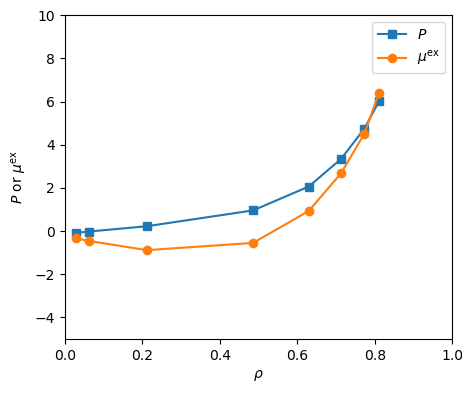
\(\mu \)VT MC. Fig. 21 shows isotherms at \(T\) = 2.0 of pressure and excess chemical potential for the LJ fluid computed
using mclg_muvt.c. These were computed using three independent trials per data point. This matches Fig. 5.8
in F&S [1].