6.2 Molecular Dynamics at Constant Temperature

Conventional MD simulation conserves total energy; hence, the time averages computed from MD simulation, if it is long enough, are equivalent to ensemble averages computed from the microcanonical ensemble. The flexibility of MD is greatly enhanced by noting that it is not restricted to NVE. There exist techniques by which MD can simulate in the NVT or NPT ensembles as well. We will consider some popular temperature control schemes, and one popular pressure control scheme, in this section.

There are essentially three ways to control the temperature in an MD simulation:

1.

Velocity rescaling;

2.

Stochastic forces and/or velocities; and

3.

“Extended Lagrangian” formalisms.

Each of these classes of schemes has advantages and disadvantages, depending on the application. In the following subsections, we consider several examples of thermostats, and attempt to discuss their advantages and drawbacks. A simple barostat is also described in the last section.

6.2.1 Temperature Fluctuations in the Canonicial Ensemble

Before considering how to fiddle with particle velocities or forces to enforce constant temperature, it is worth considering what statistical thermodynamics has to say about temperature. When we have direct knowledge of instantaneous particle velocities, we know that the kinetic energy is \begin{equation} \mathscr {K} = \sum _{i=1}^{N} \sum _{\alpha \in \left \{x,y,z\right \}}\frac {p_{i,\alpha }^2}{2m} \equiv \sum _{j=1}^{3N}\frac {p_j^2}{2m} \end{equation} where we recognize that all momentum components are independent variables. We also know that temperature (in reduced units) is directly proportional to kinetic energy: \begin{equation} \frac {3}{2}NT = \mathscr {K} \end{equation} With this equivalence, we can consider the “instantaneous” temperature as \begin{equation} T = \frac {2}{3N}\sum _{j=1}^{3N}\frac {p_j^2}{2m} \end{equation} Since momenta must fluctuate it is necessarily the case that instantaneous temperature also fluctuates. Let’s see how much.

First, since all momenta are independent, it follows from the definition of the canonical partition function that a particle momentum component \(p_j\) follows the Maxwell-Boltzmann distribution: \begin{equation} \rho (p_j) = \left (\frac {\beta }{2\pi m}\right )^{\frac 32}\exp \left (-\frac {\beta p_j^2}{2m}\right ) \end{equation} We can characterize fluctuations in \(p_j^2\) by dividing its variance \(\sigma _{p_j^2}\) to the square of its average \(\langle p_j^2\rangle ^2\). The variance is defined \begin{equation} \sigma _{p_j^2} = \langle p_j^4\rangle -\langle p_j^2\rangle \end{equation} Using the Maxwell-Boltzmann distribution: \begin{equation} \langle p_j^2\rangle = \int _{-\infty }^{\infty }dp_j p_j^2 \exp \left (-\frac {\beta p_j^2}{2m}\right ) = \frac {3m}{\beta } \end{equation} and \begin{equation} \langle p_j^4\rangle = \int _{-\infty }^{\infty }dp_j p_j^4 \exp \left (-\frac {\beta p_j^4}{2m}\right ) = 15\left (\frac {m}{\beta }\right )^2 \end{equation} Thus, \begin{equation} \frac {\langle p_j^4\rangle -\langle p_j^2\rangle }{\langle p_j^2\rangle } = \frac {2}{3}. \end{equation} Now, let’s compute fluctuations in the instantaneous temperature. First, the average: \begin{equation} \langle T\rangle = \frac {2}{3N}\sum _{j=1}^{3N}\frac {\langle p_j^2\rangle }{2m} = \frac {2}{3N}\frac {3N}{2m}\langle p_j^2\rangle = \frac {\langle p_j^2\rangle }{m} \end{equation} Now the variance, \(\langle T^2\rangle - \langle T\rangle \), starting with \(\langle T^2\rangle \): \begin{equation}\label {eq:T2a} \begin {aligned} \langle T^2\rangle &= \left (\frac {2}{3N}\right )^2\Bigg <\left (\sum _{j=1}^{3N}\frac {p_j^2}{2m}\right )\left (\sum _{k=1}^{3N}\frac {p_k^2}{2m}\right )\Bigg >\\ &= \left (\frac {2}{3N}\right )^2 \sum _{jk}\frac {\langle p_j^2p_k^2\rangle }{(2m)^2}\\ &= \left (\frac {2}{3N}\right )^2\left [9N\frac {\langle p_j^4\rangle }{(2m)^2}+9N(N-1)\frac {\langle p_j^2\rangle ^2}{(2m)^2}\right ] \end {aligned} \end{equation} \begin{equation}\label {eq:T2b} \langle T^2\rangle = \frac {1}{(mN)^2}\left [N\langle p_j^4\rangle +N(N-1)\langle p_j^2\rangle ^2\right ] \end{equation} Note that in going from Eq. 167 to 168, we note the fact that \begin{equation} \langle p_j^2p_k^2 \rangle = \langle p_j^2\rangle \langle p_k^2\rangle = \langle p_j^2\rangle ^2 \end{equation} since momenta are not correlated to each other. Putting these together: \begin{equation} \begin {aligned} \frac {\langle T^2\rangle - \langle T\rangle ^2}{\langle T\rangle ^2} & = \frac {\frac {1}{(mN)^2}\left [N\langle p_j^4\rangle +N(N-1)\langle p_j^2\rangle ^2\right )] - \left (\frac {\langle p_j^2\rangle }{m}\right )^2}{\left (\frac {\langle p_j^2\rangle }{m}\right )^2} \\ & = \frac {N\langle p_j^4\rangle +N(N-1)\langle p_j^2\rangle ^2 - N^2\langle p_j^2\rangle ^2}{N^2\langle p_j^2\rangle ^2} \\ & = \frac {1}{N}\frac {\langle p_j^4\rangle -\langle p_j^2\rangle ^2}{\langle p_j^2\rangle ^2} = \frac {2}{3N} \end {aligned} \end{equation}

So clearly temperature fluctuates in the canonical ensemble. Of course, in the thermodynamic limit (\(N\rightarrow \infty \)), these fluctuations vanish and we perceive a “constant” temperature, but in a simulation in which we resolve the momenta of a set of \(N\) particles, we must observe that \(T\) fluctuations as shown above. We can use this fact to decide whether or not a temperature-control scheme in MD is actually resulting in sampling the canonical ensemble.

6.2.2 Velocity Rescaling: Isokinetics and the Berendsen Thermostat

“Isokinetics” refers to altering velocities on the fly to keep kinetic energy (and therefore temperature) constant. The relationship between kinetic energy and temperature results from the application of the equipartition theorem to velocity (or, equivalently, momentum) degrees of freedom: \begin{align} \label {eq:veleqpart} \frac {3}{2}Nk_BT & = \frac {1}{2}\sum _im_iv_i^2m = \sum _i\frac {p_i^2}{2m} \end{align}

Scaling every particle velocity by a factor \(\lambda \) will yield a new temperature \(T^\prime \): \begin{equation} \lambda = \sqrt {\left (T^\prime /T\right )} \end{equation} An isokinetic thermostat computes \(\lambda \) and rescales velocities at every time step. Such a thermostat cannot be used to conduct a simulation in the canonical ensemble, since it totally suppresses the required temperature fluctuations. However, isokinetics is perfectly fine to use in a warmup or initialization phase in order to prevent numerical instabilities.

The code mdlj_isok.c illustrates implementation of an isokinetic thermostat for constant-\(T\) simulation of a Lennard-Jones fluid. The implementation uses a two parameters, isoKT and isoKi, that specify the desired temperature and the number of time steps between applications of the rescaling. It is worth asking whether or not occasional velocity rescaling (rather than at every step) might allow us to preserve the correct statistics. 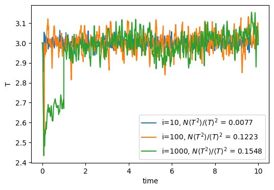Fig. 22 shows traces of temperature vs time for three MD simulations of the Lennard-Jones fluid with 512 particles at a density of 0.50. Each simulation used a different interval size i. The quantity \(N\frac {\langle T^2\rangle - \langle T\rangle ^2}{\langle T\rangle ^2}\) is computed for each set and values are shown in the legend. For pure canonical statistics, we know this should be 2/3; clearly, isokinetics even at a very modest frequency utterly fails to preserve canonical statistics.

Berendsen realized that velocity scaling could be reformulated to model energy exchange with a bath at constant \(T\) [9]. His scale factor is defined as \begin{equation} \label {eq:lam_ber} \lambda = \left [1+\frac {\Delta t}{\tau _T}\left (\frac {T_0}{T} - 1\right )\right ]^{\frac {1}{2}} \end{equation} Here, \(T_0\) is the setpoint temperature, \(\Delta t\) is the integration time step, and \(\tau _T\) is a constant called the “rise time” of the thermostat. It describes the strength of the coupling of the system to a hypothetical heat bath. The larger \(\tau _T\), the weaker the coupling; in other words, the larger \(\tau _T\), the longer it takes to achieve a given \(T_0\) after an instantaneous change from some previous \(T_0\).

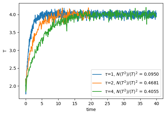
The code mdlj_ber.c implements the Berendsen thermostat. The two relevant parameters are berT, the setpoint temperature, and ber_tau, the rise time. Fig. 23 shows traces of temperature vs time for three MD simulations of the Lennard-Jones fluid with 512 particles at a density of 0.50, with temperature controlled using the Berendsen thermostat with various values of \(\tau \). Larger \(\tau \) clearly results in longer approach times to the setpoint temperature. Note also that the relative fluctuations of the temperature reported indicate that canonical statistics are not being held.

Though relatively simple, velocity scaling thermostats are not recommended for use in production MD runs because they do not strictly conform to the canonical ensemble.

6.2.3 Stochastic NVT Thermostats: Andersen, Langevin, and Dissipative Particle Dynamics

The Andersen Scheme. Perhaps the simplest thermostat which does correctly sample the NVT ensemble is due to Andersen [10]. Here, at each step, some prescribed number of particles is selected, and their momenta (actually, their velocities) are drawn from a Gaussian distribution at the prescribed temperature (otherwise known as the Maxwell-Boltzmann distribution): \begin{equation} \label {eq:ens:gaus} \mathscr {P}(p) = \left (\frac {\beta }{2\pi m}\right )^{3/2} \exp \left [-\beta p^2/\left (2m\right )\right ] \end{equation} This is intended to mimic collisions with bath particles at a specified \(T\). The strength of the coupling to the heat bath is specified by a collision frequency, \(\nu \). For each particle, a random variate is selected between 0 and 1. If this variate is less than \(\nu \Delta t\), then that particle’s momenta are reset.

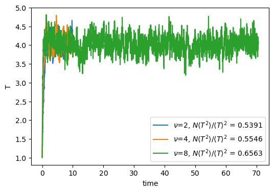
The code mdlj_and.c implements the Andersen thermostat for the Lennard-Jones fluid. The two relevant parameters are and_T, the setpoint temperature, and and_nu, the rise time. Fig. 24 shows traces of temperature vs time for three MD simulations of the Lennard-Jones fluid with 512 particles at a density of 0.50, with temperature controlled using the Andersen thermostat with various values of collision frequency \(\nu \). Larger \(\nu \) results in longer approach times to the setpoint temperature, but it is also clear that for these values of \(\nu \), the Andersen thermostat acts much more quickly than the Berendsen thermostat. Note also that the relative fluctuations of the temperature reported indicate that canonical statistics are in fact being held.

Although temperature fluctuations match the canonical ensemble, the Andersen thermostat destroys momentum transport because of the random reassignment of velocities; hence, there is no continuity of momentum in an Andersen LJ fluid, and therefore no proper \(\mathscr {D}\) or viscosity. Fig. 6.3 in Frenkel & Smit clearly shows that \(\mathscr {D}\), if measured from an Andersen MD run, is incorrect.

The Langevin thermostat. In the “Langevin” thermostat, at each time step all particles receive a random force and have their velocities lowered using a constant friction. [11] The average magnitude of the random forces and the friction are related in a particular way, which guarantees that the “fluctuation-dissipation” theorem is obeyed, thereby guaranteeing NVT statistics.

In this formalism, the particle-\(i\) equation of motion is modified: \begin{equation} \label {ens:md:lang} m\ddot {\bf r}_i = -\nabla _i U - m\Gamma \dot {\bf r}_i + {\bf W}_i\left (t\right ) \end{equation} Here, \(\Gamma \) is a friction coefficient with units of \(\tau ^{-1}\), and \({\bf W}_i\) is a random force that is uncorrelated in time and across particles, with a mean given by \begin{equation} \left <{\bf W}_i\left (t\right ),{\bf W}_j\left (t^\prime \right )\right > = \delta _{ij}\delta \left (t-t^\prime \right )6k_BmT\Gamma \end{equation}

The code mdlj_lan.c implements the Langevin thermostat. The two relevant parameters are lanT, the setpoint temperature, and lan_friction, the friction \(\Gamma \). The two major elements are a force initialization at each time step that adds in the random forces, \(\bf W\), and a slight modification to the update equations in the integrator to include the effect of \(\Gamma \). Note that the initialization of forces to zero in the force routine has been removed.

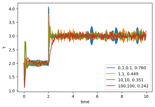
Fig. 25 shows temperature vs time for several MD simulations of a 512-particle LJ fluid at a density of 0.5; the upper plot shows data from runs with \(\Delta t\)=10\(^{-3}\), and the lower plot \(\Delta t\)=10\(^{-2}\), each showing four values of \(\Gamma \). Relative temperature fluctuations indicate weak agreement with canonical statistics that improves for the lower values of \(\Delta t\).

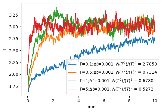
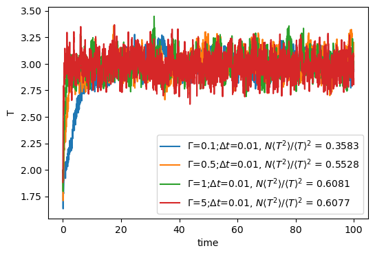
One advantage of the Langevin thermostat (and to a limited extent, the Andersen thermostat and other stochastic-based thermostats) is that we can get away with a larger time step than in NVE simulations. At a density of \(\rho \) = 0.8442 and a mean temperature \(T\) = 1.0, an NVE simulation is unstable for time-steps above about \(\Delta t\) = 0.004. We can, however, run a Langevin dynamics simulation with a friction \(\Gamma \) = 1.0 stably with a time-step as large as \(\Delta t\) = 0.01 or even higher. This has proven invaluable in simulations of more complicated systems that simple liquids, namely linear polymers, which have very long relaxation times. MD with the Langevin thermostat is the method of choice for equilibrating samples of liquids of long bead-spring polymer chains.

Of course, the drawback of most stochastic thermostats (one exception is discussed next) is that momentum transfer is destroyed. So again, it is unadvisable to use Langeving or Andersen thermostats for runs in which you wish to compute diffusion coefficients. The recommendation stands: use NVE to compute properties, and use thermostats for equilibration only.

The Dissipative Particle Dynamics thermostat. The DPD thermostat [12, 13] adds pairwise random and dissipative forces to all particles, and has been shown to preserve momentum transport. Hence, it is the only stochastic thermostat so far that should even be considered for use if one wishes to compute transport properties.

The DPD thermostat is implemented by slight modification of the force routine to add in the pairwise random and dissipative forces. For the \(ij\) pair, the dissipative force is defined as \begin{equation} {\bf f}_{ij}^D = -\gamma \omega ^D\left (r_{ij}\right )\left ({\bf v}_{ij}\cdot \hat {\bf r}_{ij}\right )\hat {\bf r}_{ij} \end{equation} Here, \(\gamma \) is a friction coefficient, \(\omega \) is a cut-off function for the force as a function of the scalar distance between \(i\) and \(j\) which simply limits the interaction range of the dissipative (and random) forces, \({\bf v}_{ij} = {\bf v}_i - {\bf v}_j\) is the relative velocity of \(i\) to \(j\), and \(\hat {\bf r}_{ij} = {\bf r}_{ij}/r_{ij}\) is the unit vector pointing from \(j\) to \(i\). The random force is defined as \begin{equation} {\bf f}_{ij}^R = \sigma \omega ^R\left (r_{ij}\right )\zeta _{ij}\hat {\bf r}_{ij} \end{equation} Here, \(\sigma \) is the strength of the random force, \(\omega ^R\) is a cut-off, and \(\zeta _{ij}\) is a Gaussian random number with zero mean and unit variance, and \(\zeta _{ij} = \zeta _{ji}\).

The update of velocity uses these new forces: \begin{equation} \label {eq:dpd_update} {\bf v}_i\left (t + \Delta t\right ) = {\bf v}_i\left (t\right ) - \frac {\Delta t}{m}\nabla _iU + \frac {\Delta t}{m}{\bf f}_i^D + \frac {\sqrt {\Delta t}}{m}{\bf f}_i^R \end{equation} where \begin{equation} \begin {aligned} {\bf f}_i^D & = \sum _{j\ne i} {\bf f}_{ij}^D \\ {\bf f}_i^R & = \sum _{j\ne i} {\bf f}_{ij}^R \end {aligned} \end{equation}

The parameters \(\gamma \) and \(\sigma \) are linked by a fluctuation-dissipation theorem: \begin{equation} \sigma ^2 = 2\gamma k_B T \end{equation} So, in practice, one must specify either \(\gamma \) or \(\sigma \), and then a setpoint temperature, \(T\), in order to use the DPD thermostat.

The cutoff functions are also related: \begin{equation} \omega ^D\left (r_{ij}\right ) = \left [\omega ^R\left (r_{ij}\right )\right ]^2 \end{equation} This is the only real constraint on the cutoffs; we are otherwise allowed to use any cutoff we like. The simplest uses the cutoff radius of the pair potential, \(r_c\): \begin{equation} \omega \left (r\right ) = \begin {cases} 1 & r < r_c\\ 0 & r > r_c \end {cases} \end{equation} Note that, with this choice, \(\left [\omega ^R\left (r_{ij}\right )\right ]^2\) = \(\omega ^R\left (r_{ij}\right )\) = \(\omega ^D\left (r_{ij}\right ) = \omega \).

The code mdlj_dpd.c implements the DPD thermostat in an MD simulation of the Lennard-Jones liquid. The major changes (compared to mdlj.c) are to the force routine, which now requires several more arguments, including particle velocities, and parameters for the thermostat. Inside the pair loop, the force on each particle is updated by the conservative, dissipative, and random pairwise force components. The random force is divided by \(\sqrt {\Delta t}\) so that the velocity Verlet algorithm need not be altered to implement Eq. 179.

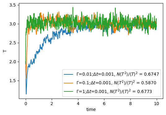
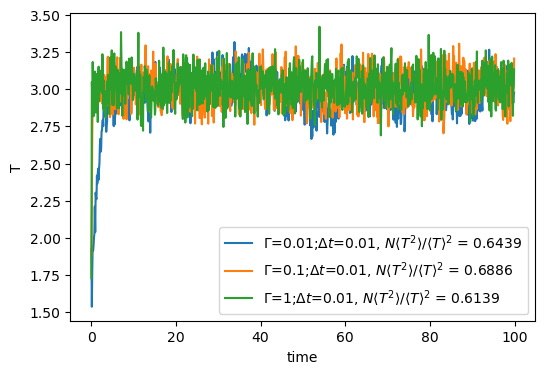
The behavior of the DPD thermostat can be assessed in a similar fashion as was the Berendsen thermostat above. Here I’ve run several MD simulations of the LJ fluid at a density of 0.84 with 512 particles for 10,000 steps, with various values of \(\Gamma \) and \(\Delta t\). Fig. 26 shows the temperature vs time for these various runs. We see that increased friction leads to faster approach to the setpoint temperature, and that temperature fluctuations seem to conform to canonical statistics pretty well.

6.2.4 The Nosé-Hoover Chain

The final thermostat we consider is one based on the extended Lagrangian formalism, which leads to a deterministic trajectory; i.e., there are no random forces or velocities to deal with. The most common and so far most reliable thermostat of this kind is the Nosé-Hoover thermostat. This thermostat can be implemented as a “single” or a “chain”; here, we consider a chain.

The basic idea of the Nosé-Hoover thermostat is to use a friction factor to control particle velocities. This friction factor is actually the scaled velocity, \(v_{\xi _1}\), of an additional and dimensionless degree of freedom, \(\xi _1\). This degree of freedom has an associated “mass”, \(Q_1\), which effectively determines the strength of the thermostat. The equations of motion obeyed by this additional degree of freedom guarantee that the original degrees of freedom (\({\bf r}^N\), \({\bf p}^N\)) sample a canonical ensemble. This degree of freedom is the terminus of a chain of similar degrees of freedom, each with their own mass. The chain has a total of \(M\) “links.” The overall set of equations of motion are:

The main advantage of the Nosé-Hoover chain thermostat is that the dynamics of all degrees of freedom are deterministic and time-reversible. No random numbers are used. The code mdlj_nhc.c implements an \(M\) = 2 Nosé-Hoover chain thermostat in an MD simulation of an Lennard-Jones fluid, by implementing Algorithms 30, 31, and 32 from Frenkel & Smit. The relevant parameters are nhcT, the setpoint temperature, and nhcQ, the two masses. Fig. 27 illustrates the use of the NHC thermostat on an N=512, \(\rho \) = 0.84 LJ system.