5.4 Case Study 3: Transport Properties: The Self-Diffusion Coefficient
This Case Study combines elements of Case Studies 5 and 6 in F&S, which are unfortunately incomplete in their description. The purpose of this Case Study is to demonstrate how one computes a self-diffusion coefficient, \(\mathscr {D}\), from an MD simulation of a simple Lennard-Jones liquid. There are two means to computing \(\mathscr {D}\): (1) the mean-squared displacement (“MSD”) \(\left <r^2\right >(t)\), and (2) the velocity autocorrelation function, \({\rm VACF}(t)\). The approaches are equivalent in the sense that the MSD is the integral representation of the VACF; the former is termed the “Einstein” approach, while the latter is the “Green-Kubo” approach [8].
The self-diffusion coefficient governs the evolution of concentration, \(c\), (or number density) according to a generalized transport equation: \begin{equation} \frac {\partial c}{\partial t} = \mathscr {D}\nabla ^2c \end{equation} Einstein showed (details in text) that \(\mathscr {D}\) is related to the mean-squared displacement, \(\left <r^2\right >\): \begin{equation} \label {eq:md:ein} \frac {\partial \left <r^2\right >}{\partial t} = 6\mathscr {D} \end{equation} At long times, \(\mathscr {D}\) should be independent of time; hence \begin{equation} \left <r^2\right > = \lim _{t\rightarrow \infty }6\mathscr {D}t \end{equation} We can compute \(\left <r^2\right >\), and therefore estimate \(\mathscr {D}\), easily using MD simulation. There is, however, a very important consideration concerning periodic boundary conditions. Recall that, during integration, immediately after the position update, we test to see if the update has taken the particle outside of the primary box. If it has, we simply shift the particle’s position by a box length in the appropriate dimension and direction. The displacement of the particle during this step is not a box length, but if you consider just the coordinates as they appear in the output, you would think that it is. It is therefore important that we work with unfolded coordinates when computing mean-squared displacement. This is not adequately explained in the text, so we cover it in some detail here.
“Unfolding” coordinates in a simulation with periodic boundaries requires that we keep track of how many
times each particle has crossed a boundary. The code mdlj.c allows output of unfolded coordinates in the
trajectory output using the -uf switch on the command line. Now, generally the array rx[] always contains the
periodically shifted coordinates, but we can easily generate the unfolded coordinates at any time (say, upon
output) by performing the following operation:
rxu = rx[i]+ix[i]*L;
This is because ix[] contains a tally of the number of times periodic crossings in the \(x\) direction have occurred:
+1 is added to the tally every time a particle’s \(x\) position exceeds \(L\) and is wrapped back in by subtracting \(L\), and -1
is added to the tally every time a particle’s \(x\) position is below 0 and is wrapped back in by adding \(L\). Here, \(L\) is the
box length (assumed cubic).
The program msd.c computes the MSD from a trajectory with unfolded coordinates using a
conventional, straightforward algorithm. The C-code for this algorithm appears below. \(M\) is the number of
“frames” in the trajectory, and \(N\) is the number of particles. \(\left <r^2\right >(t)\) is computed by considering the change in
particle position over an interval of size \(t\). Any frame in the trajectory can be considered an origin
for any interval size, provided enough frames come after it in the trajectory. This means that we
additionally average over all possible time origins. dt is a variable that loops over allowed time
intervals. cnt[] counts the number of time origins for a given interval. sd[] is the array in which we
accumulate squared displacement at each time interval, and has \(M\) elements, one for each allowed
interval.
/* Compute the mean-squared displacement using
   the straightforward algorithm */
fprintf(stdout,"# computing MSD...\n");fflush(stdout);
for (t=begin_frame;t<M;t++) {
    for (dt=1;(t+dt)<M;dt++) {
        cnt[dt]++;  /* number of origins for interval length dt  */
        for (i=0;i<Traj[0]->N;i++) {
            sd[dt] += rij2_unwrapped(Traj[t+dt],i,Traj[t],i,1);
        }
    }
}
The function rij2_unwrapped(fi,i,fj,j,1) very simply computes the squared displacement between
particle i in frame fi and particle j in frame fj:
double rij2_unwrapped ( frametype * fi, int i,
                        frametype * fj, int j, int com_corr ) {
    double dx, dy, dz;
    dx=fi->rx[i]-(com_corr?fi->cx:0)-fj->rx[j]+(com_corr?fj->cx:0);
    dy=fi->ry[i]-(com_corr?fi->cy:0)-fj->ry[j]+(com_corr?fj->cy:0);
    dz=fi->rz[i]-(com_corr?fi->cz:0)-fj->rz[j]+(com_corr?fj->cz:0);
    return dx*dx+dy*dy+dz*dz;
}
The parameter com_corr removes the center of mass drift from the displacement; the center of mass should
not move in NVE, but we will use this code for trajectories in which the COM does diffuse. The center of mass
of a frame is part of the frametype data type used in msd.c, and it’s computed when the frame is read
in.
The code fragment below completes the averaging, and outputs the total mean-squared displacement.
fp=fopen(outfile,"w");
fprintf(fp,"# MSD from %s\n",trajfile);
fprintf(fp,"#LABEL time msd\n");
fprintf(fp,"#UNITS %s %s^2\n",time_units,length_units);
for (t=0;t<M-begin_frame;t++) {
    sd[t] /= cnt[t]?(Traj[0]->N*cnt[t]):1;
    fprintf(fp,"% .5lf % .8lf\n",
        t*traj_interval*md_time_step,sd[t]);
}
fclose(fp);
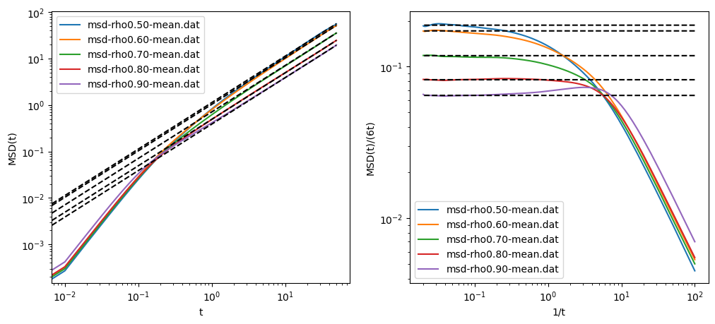
Fig. 18 shows MSD vs time from 60,000-step MD simulations at various densities in which frames are
saved at intervals of 10 time-steps. In these simulations, the density was constant and there were 216 particles,
with velocities initialized at 0.7. The figure shows the data plotted two ways: MSD vs. \(t\) on the left, and MSD/(6\(t\))
vs 1/\(t\) on the right. The program msd can post-process an unwrapped trajectory file to generate the
MSD:
$ ./msd -t traj-rho0.90-rep0.xyz -traj-interval 10 \
  -o msd-rho0.90-rep0.dat -begin-frame 1000
Repeating this process for several densities and several replicas per density builds a nice dataset. MSD at
each density was averaged over replicas and plotted using plot_msd.py:
$ python ../../../originals/plot_msd.py -i msd-rho0.50-mean.dat \
  -i msd-rho0.60-mean.dat -i msd-rho0.70-mean.dat \
  -i msd-rho0.80-mean.dat -i msd-rho0.90-mean.dat  \
  -o msd-rho-T0.70.png -lowt 1
msd-rho0.50-mean.dat 0.18750243355919102
msd-rho0.60-mean.dat 0.17188252756031633
msd-rho0.70-mean.dat 0.11801146782479009
msd-rho0.80-mean.dat 0.08188412712076683
msd-rho0.90-mean.dat 0.0645241901384243
The parameter -lowt is the lower time limit beyond which the data is fit to calculate \(\mathscr {D}\). Values of \(\mathscr {D}\) are output
here.
You can see that the MSD transitions from a short-time regime where MSD \(\propto \) t\(^2\) to a long-time regime where MSD \(\propto \) t. That short-time region displays “ballistic” behavior, and on those time scales particles move ballistically (with constant velocity) between collisions with other particles; you can see by the value of MSD of about 0.02 that they are moving only about 0.1 particle diameters or so before colliding. On the longer, “diffusive” timescales, we can see the expected behavior.
The velocity autocorrelation function route to the diffusion constant begins with the realization that one can reconstruct the displacement of a particle over a time interval \(t\) by simply integrating its velocity: \begin{equation} \Delta {\bf r} = \int _0^t {\bf v}(t^\prime )dt^\prime \end{equation} So, the mean squared displacement can be expressed \begin{equation} \begin {aligned} \left <r^2\right > & = \left <\left (\int _0^t{\bf v}(t^\prime )dt^\prime \right )^2\right > \\ & = \int _0^t\int _0^t dt^\prime dt^{\prime \prime } \left <{\bf v}(t^\prime )\cdot {\bf v}(t^{\prime \prime })\right > \\ & = 2\int _0^t\int _0^{t^\prime } dt^\prime dt^{\prime \prime } \left <{\bf v}(t^\prime )\cdot {\bf v}(t^{\prime \prime })\right >. \end {aligned} \end{equation} The third equality arises because we can swap \(t^\prime \) and \(t^{\prime \prime }\). The quantity \( \left <{\bf v}(t^\prime )\cdot {\bf v}(t^{\prime \prime })\right >\) is the velocity autocorrelation function. This is an example of a Green-Kubo relation; that is, a relation between a transport coefficient, and an autocorrelation function of a dynamical variable. Eq. 138 then leads to \begin{equation}\label {eq:gkD} \mathscr {D} = \frac {1}{3}\int _0^\infty \left <{\bf v}(t^\prime )\cdot {\bf v}(t^{\prime \prime })\right > dt \end{equation} So, the second route to computing \(\mathscr {D}\) requires that we numerically integrate \(\left <{\bf v}(t^\prime )\cdot {\bf v}(t^{\prime \prime })\right >\) out to very large times. How large? First, let’s try to understand the behavior of \(\left <{\bf v}(t^\prime )\cdot {\bf v}(t^{\prime \prime })\right >\).
In three dimensions, we compute this by computing the components and adding them together, as we did for mean-squared displacement: \begin{equation} \left <{\bf v}(t^\prime )\cdot {\bf v}(t^{\prime \prime })\right > = \left <v_x(t^\prime )v_x(t^{\prime \prime })\right >+ \left <v_y(t^\prime )v_y(t^{\prime \prime })\right >+ \left <v_z(t^\prime )v_z(t^{\prime \prime })\right > \end{equation} The code to compute the VACF is essentially identical to that for the MSD, with the exception that the quantity we accumulate is the dot product of velocity vectors:
/* Compute velocity dot product between particles i and j in
   frame fi and fj, respectively; com_corr removes center of
   mass motion */
double vij2 ( frametype * fi, int i, frametype * fj, int j,
              int com_corr ) {
    double dx, dy, dz;
    dx=(fi->vx[i]-(com_corr?fi->cvx:0))*(fj->vx[j]-(com_corr?fj->cvx:0));
    dy=(fi->vy[i]-(com_corr?fi->cvy:0))*(fj->vy[j]-(com_corr?fj->cvy:0));
    dz=(fi->vz[i]-(com_corr?fi->cvz:0))*(fj->vz[j]-(com_corr?fj->cvz:0));
    return dx+dy+dz;
}
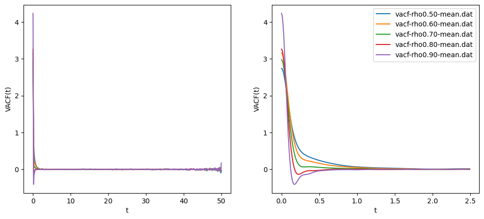
Fig. 19 shows the VACF for the same simulation we showed for the MSD above. The right panel is a zoom in
by a factor of 20, which allows us to resolve the part of the VACF that dips below zero at short times; this is the
same time scale on which we have ballistic motion. The negative VACF indicates “bounce-back” from
collisions. That figure was generated using plot_vacf.py, which also applies Eq. 142 using
scipy.integrate.simpson() to compute \(\mathscr {D}\)’s:
$ python ../../../originals/plot_vacf.py -i vacf-rho0.50-mean.dat \
  -i vacf-rho0.60-mean.dat -i vacf-rho0.70-mean.dat \
  -i vacf-rho0.80-mean.dat -i vacf-rho0.90-mean.dat \
  -o vacf-rho-T0.70.png -z 20
vacf-rho0.50-mean.dat 0.16226338888888892
vacf-rho0.60-mean.dat 0.16724698888888884
vacf-rho0.70-mean.dat 0.11846137777777778
vacf-rho0.80-mean.dat 0.08435750000000004
vacf-rho0.90-mean.dat 0.0705403444444444
These values agree only weakly with the values computed via fitting to MSD, but either is considered “correct”.