The Method of Overlapping Distributions

10.3 The Method of Overlapping Distributions

One interesting feature of the Widom method is that the only trial move is insertion; however, the free-energy difference between an \(N\)-particle system and an \(N+1\)-particle system should not depend on which direction the trial moves take. If we imagine a “Widom real-particle removal” method, we’d write the chemical potential as

\begin{align} \mu & = +k_BT\ln \left (Q_N/Q_{N+1}\right ) = \mu _{\rm id} + k_BT\ln \langle \exp \left (+\beta \Delta \mathscr {U}\right )\rangle \end{align}

Sampling \(\langle \exp \left (+\beta \Delta \mathscr {U}\right )\rangle \) in a straightforward NVT MC simulation won’t work, however, because...

There is, however, a right way to use bidirectional energy changes to compute free-energy differences, termed the “overlapping distribution method” and attributed to Bennett [44]. Consider two systems 0 and 1, obeying potentials \(\mathscr {U}_0\) and \(\mathscr {U}_1\), respectively. Let \(q_i\) be the scaled configurational integral of the Boltzmann factor:

\begin{equation} q_i = \int d{\uu {s}^N} e^{-\beta \mathscr {U}_i} \end{equation}

We can then express the free energy difference between these systems as (assuming for simplicity they have the same volumes):

\begin{equation} \beta \Delta F = -\ln \frac {q_1}{q_0} \end{equation}

Consider next we run an NVT MC simulation on \(\mathscr {U}_1\) and sample \(\Delta \mathscr {U}\equiv \mathscr {U}_1-\mathscr {U}_0\). Formally, the probability density of \(\Delta \mathscr {U}\) from this simulation is

\begin{equation}\label {eq:od:gym1} p_1(\Delta \mathscr {U}) = \frac {\ds \int d{\uu {s}^N} e^{-\beta \mathscr {U}_1}\delta (\mathscr {U}_1-\mathscr {U}_0-\Delta \mathscr {U})}{q_1} = \frac {\ds \int d{\uu {s}^N} e^{-\beta (\mathscr {U}_0+\Delta \mathscr {U})}\delta (\mathscr {U}_1-\mathscr {U}_0-\Delta \mathscr {U})}{q_1} \end{equation}

\begin{equation}\label {eq:od:gym2} p_1(\Delta \mathscr {U}) = \frac {q_0}{q_1}e^{-\beta \Delta \mathscr {U}}\frac {1}{q_0}\int d\uu {s}^Ne^{-\beta \mathscr {U}_0}\delta (\mathscr {U}_1-\mathscr {U}_0-\Delta \mathscr {U}) = \frac {q_0}{q_1}e^{-\beta \Delta \mathscr {U}}p_0(\Delta \mathscr {U}) \end{equation} In going from Eq. 261 to 262 we have used the fact that the Dirac delta function will only permit one value of \(\Delta \mathscr {U}\) to survive integration. Taking the log of both sides gives \begin{equation} \begin {aligned} \ln p_1(\Delta \mathscr {U}) &= -\ln \frac {q_1}{q_0} - \beta \Delta \mathscr {U} + \ln p_0(\Delta \mathscr {U}) \\ & = \beta (\Delta F - \Delta \mathscr {U}) + \ln p_0(\Delta \mathscr {U}) \end {aligned} \end{equation} This equation provides a way to estimate \(\Delta F\) at any one value of \(\Delta \mathscr {U}\) so long as good estimates of both \(p_1(\Delta \mathscr {U})\) and \(p_0(\Delta \mathscr {U})\) are available. That means we must be able to sample a sufficiently large domain of \(\Delta \mathscr {U}\) from both a simulation run on \(\mathscr {U}_1\) and another run on \(\mathscr {U}_0\). That is, there must be a domain of \(\Delta \mathscr {U}\) where \(p_1\) and \(p_0\) overlap.

Bennett[44] suggests the following transformation of \(p_1\) and \(p_0\) to permit easy calculation of \(\Delta F\). Letting \begin{equation} \begin {aligned} f_0(\Delta \mathscr {U}) & \equiv \ln p_0(\Delta \mathscr {U}) - \frac {\beta \Delta \mathscr {U}}{2},\ \ \mbox {and} \\ f_1(\Delta \mathscr {U}) & \equiv \ln p_1(\Delta \mathscr {U}) + \frac {\beta \Delta \mathscr {U}}{2} \end {aligned} \end{equation} gives \begin{equation} \beta \Delta F = f_1(\Delta \mathscr {U})-f_0(\Delta \mathscr {U}). \end{equation} This means we can measure \(f_1\) and \(f_0\) in separate simulations, and then observe a constant offset between them to be \(\beta \Delta F\).

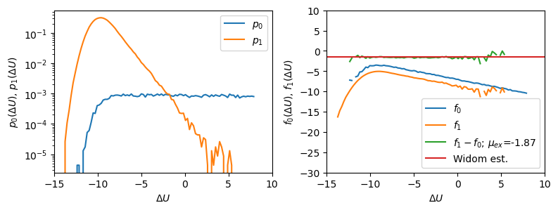
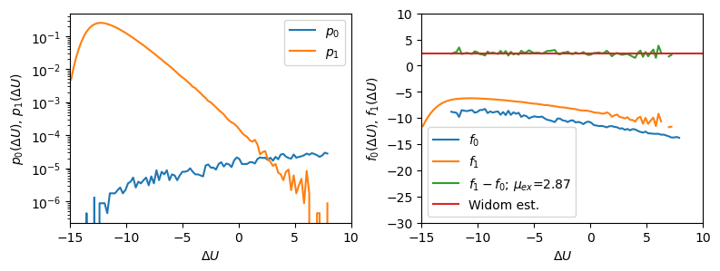
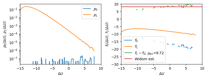
Suppose we now take the example of system 1 with \(N\) real particles and system 0 with \(N-1\) real particles and one ideal-gas particle. The free-energy change from 0 to 1 is the excess chemical potential (yet again!). Fig. 41 illustrates using Bennett’s method to compute \(\mu _{\rm ex}\) of the Lennard-Jones fluid at \(T\) = 1.2 for a few different densities. For each density, two simulations were run: simulation-0 computes the distribution of \(\Delta \mathscr {U}\), the energy associated with converting the ideal-gas particle to a real particle, while simulation-1 computes the same distribution for converting a randomly chosen particle from being an ideal-gas particle to being a real particle. This latter \(\Delta \mathscr {U}\) is easily computed using the single-particle energy function e_i. It is important to note that the direction of the \(\Delta \) is from ideal-gas to real for both simulations. Note too that since we sample \(\Delta {\mathscr {U}}\) for particle insertion in simulation-0, we can just as easily compute the expectation \(\langle \exp (-\beta \Delta \mathscr {U})\rangle \) and thereby get a direct estimate of \(\beta \mu _{\rm ex}\).

At the moderately low density of \(\rho \) = 0.7, we see a clear constant offset \(\beta \mu _{\rm ex}\) between \(f_0\) and \(f_1\). Note clear agreement between the offset over a finite-size domain of \(\mathscr \Delta {U}\) and the single-point Widom estimate. For the somewhat higher density of 0.9, the offset is a bit noisier, reflecting somewhat poorer sampling. For the highest density, the sampling in simulation-0 is so poor that it is nearly impossible to detect an overlap domain.

Figure 41: \(p_0\) and \(p_1\) vs \(\Delta \mathscr {U}\) (left), and \(f_0\), \(f_1\), \(f_1\) - \(f_0\) vs \(\Delta \mathscr {U}\) (right) computed using NVT MC simulations at \(T\) = 1.2 of system-0 and system-1, for densities of 0.7 (top), 0.9 (middle), and 1.0 (bottom). Estimates of \(\beta \mu _{\rm ex}\) from Widom test-particle insertion are shown as red horizontal lines in the plots on the right.

← Previous Contents Next →