Adaptive Free-Energy Methods

10.5 Adaptive Free-Energy Methods

The histogram reweighting approach has a lot of parameters that have to be optimized in order to generate a reliable \(F\): the number of windows, the spring constant for the window potentials, how the windows are spaced, how much sampling in each window, and more. This is often a problem because without knowing something about \(F\) it is hard to guess the best set of WHAM parameters. This has led to the development of “adaptive” approaches that aim to overcome this supposed weakness of histogram reweighting.

The two most well-known adaptive biasing approaches are metadynamics [46] and the adaptive-biasing forces (ABF) method [47].

10.5.1 Metadynamics

10.5.1.1 Original Metadynamics In metadynamics, a time-dependent bias potential is “grown” during the course of the simulation that acts to enhance sampling of the order parameter [48]. Rather than confining to local regions of order parameter space as in umbrella sampling, the metadynamics potential pushes the system away from easily sampled regions of order parameter space. This bias can be expressed:

\begin{equation} \label {eq:metadynamics} V_b(\theta ,t) = w\sum _{t^\prime < t} \exp \left (-\frac {\left [\theta (t^\prime )-\theta (t)\right ]^2}{2\sigma ^2}\right ) \end{equation}

Here, \(w\) is a weight of each Gaussian kernel deposited, and \(\sigma \) is its width. Apart from them, another key parameter in running metadynamics is how frequently a new Gaussian kernel is added, i.e., what is the list of values for \(t^\prime \)? Apart from an irrelevant constant, the free energy along the order parameter is the time-average of the bias potential \begin{equation} \label {eq:metadynamics-f} F(\theta ) = -\frac {1}{t_f-t_i}\sum _{t=t_i}^{t_f}V_b\left [\theta (t)\right ] \end{equation}

NAMD includes native support for metadynamics using the colvars module. By default, kernels are deposited every 1,000 steps. To illustrate metadynamics, we return to the system of a single molecule of butane, this time at 273 K. It requires a 100-million time-step MD simulation to generate a smooth histogram for the C1-C4 distance at this temperature. Fig. 46 shows the free energy vs C1-C4 distance computed using a 10-million time-step metadynamics simulation for which \(w\) = 0.1 kcal/mol, and \(\sigma \) = 0.1 Å. We see excellent reconstruction of the true free energy at a much lower computational cost with metadynamics.

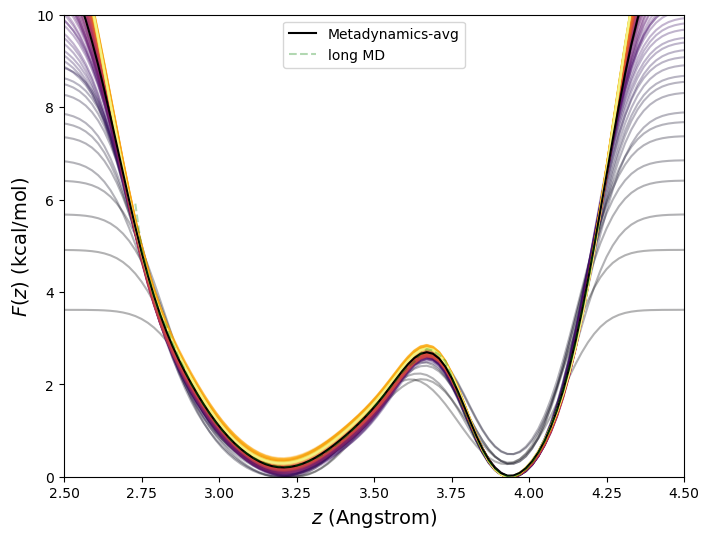
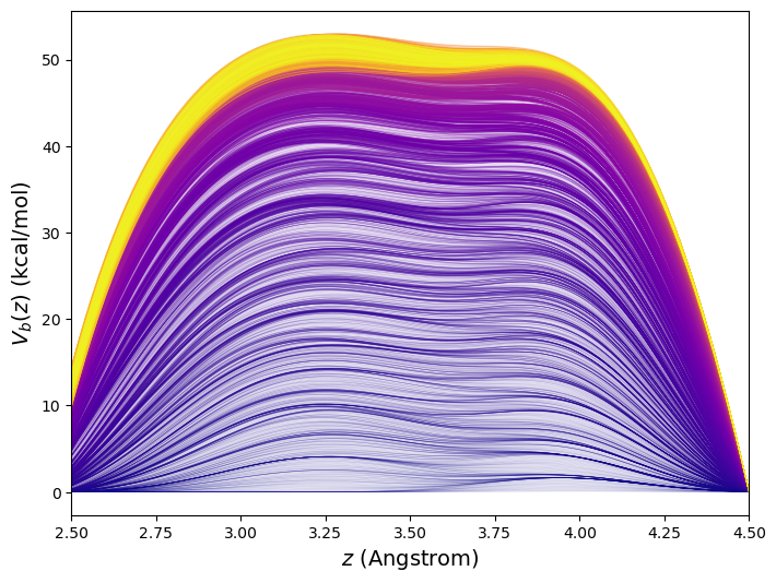
Figure 46: Free energy in kcal/mol vs. C1-C4 distance in Å, for butane in vacuum at 273 K computed using MD (green dash) and metadynamics (black solid). The MD simulation was run for 10\(^8\) timesteps, and the metadynamics for 10\(^7\). Intermediate values of the metadynamics free energy are also shown color-coded from purple (early) to yellow (late). The final metadynamics free energy is the average over all free-energy snapshots (i.e., it is the time-average negative bias potential).

This 10\(^7\)-time-step metadynamics simulation deposited 10,000 Gaussian kernels in total. Generally, it is most efficient for the simulation to keep track of the bias potential on a grid rather than as an explicit sum of Gaussians. Here, the order-parameter line was divided into increments of 0.02 Å between 1.5 and 5.5 Å, or roughly 400 points. Fig. 47 shows the evolution of the bias potential \(V_b(t)\) from this simulation.

Figure 47: Evolution of the bias potential from the 10\(^7\)-step metadynamics simulation of butane along the C1-C4 distance. The instantaneous bias potential is drawn every 10\(^5\) time-steps and shifted to its current minimum value. Each curve is drawn with an \(\alpha \) of 0.2, so where the curves appear opaque signifies a temporarily static portion of the bias as kernels are being deposited elsewhere.

The accuracy of metadynamics is fairly sensitive to \(w\) and \(\sigma \). We computed free energies for the butane system at 273 K using metadynamics (and the long MD for reference) for various combinations of \(w\) and \(\sigma \), all for 10\(^7\) steps. Among those considered, it appears \(w\) = 0.1 kcal/mol, and \(\sigma \) = 0.1 Å are the best choices. Generally, smaller \(w\) will yield more accurate free energies, but at larger computational cost.

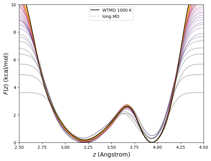
10.5.1.2 Well-Tempered Metadynamics In the well-tempered variant [49] of metadynamics, The weight \(w\) is augmented with a Boltzmann factor that diminishes exponentially as \(V_b\) builds up: \begin{equation} \label {eq:wtmd} V_b(\theta ,t) = w\sum _{t^\prime < t}\exp \left [-\frac {V_b(\theta (t^\prime ))}{\Delta T}\right ] \exp \left (-\frac {\left [\theta (t^\prime )-\theta (t)\right ]^2}{2\sigma ^2}\right ) \end{equation} \(\Delta T\) is the so-called “bias temperature”, and it acts to diminish the contribution to \(V_b\) at any \(\theta \) as time progresses, leading to a converged bias potential. The free energy is reconstructed by an inversion of the converged bias potential that requires the bias temperature: \begin{equation} \label {eq:wtmd-f} F = -\frac {T+\Delta T}{\Delta T}V_b \end{equation} Fig. 48 shows the free energy vs. C1-C4 distance for butane at 273 K computed using well-tempered metadynamics with parameters identical to the standard metadynamics run of the previous section but with a bias temperature of 1000 K.

Figure 48: Free energy in kcal/mol vs. C1-C4 distance in Å, for butane in vacuum at 273 K computed using MD (green dash) and well-tempered metadynamics (black solid). The MD simulation was run for 10\(^8\) timesteps, and the metadynamics for 10\(^7\). The bias temperature for well-biased metadynamics was 1000 K. Intermediate values of the metadynamics free energy are also shown color-coded from purple (early) to yellow (late). The final metadynamics free energy is the average over all free-energy snapshots (i.e., it is the time-average negative bias potential).

10.5.2 ABF

The adapative biasing force method is based on recovery of free energies as functions of order parameters via thermodynamic integration of mean forces. These mean forces are traditionally computed using MD simulations restrained (or constrained, depending) to particular values of the order parameter. Indeed, one way of doing this is tethering the system to a reference point with a harmonic bias potential, just as we did for the histogram reweighting approach above. In the TI formalism, however, it can be shown that the gradient of the free energy along order parameter is

Fig. 49 shows the evolution of the PMF, along with the order-parameter histogram and free-energy gradients, from a single ABF simulation of butane at 273 K using NAMD.

Figure 49: Potentials of mean force converging to a final form in an ABF simulation of butane at 273 K, where the order parameters \(z\) is the C1-C4 distance. Insets show the histogram of \(z\) (top) and the convergence of the free-energy gradients (bottom).

← Previous Contents Next →