5.2 Case Study 1: An MD Code for the Lennard-Jones Fluid
5.2.1 Introduction
Let us consider a few of the important elements of any MD program:
- 1.
- Force evaluation;
- 2.
- Integration; and
- 3.
- Configuration output.
We will understand these elements by manipulating an existing simulation program that implements the
Lennard-Jones fluid (which you may recall was analyzed using Metropolis Monte-Carlo simulation in Sec. 4).
The program is called mdlj.c in the instructional codes repository.
Recall the Lennard-Jones pair potential: \begin{equation} \label {eq:md:lj} u\left (r\right ) = 4\epsilon \left [\left (\frac {\sigma }{r}\right )^{12}- \left (\frac {\sigma }{r}\right )^{6}\right ] \end{equation} When implementing this in an MD code, similar to its implementation in MC, we adopt a reduced unit system, in which we measure length in \(\sigma \), and energy in \(\epsilon \). Additionally, for MD, we need to measure mass, and we adopt units of particle mass, \(m\). This convention makes the force on a particle numerically equivalent to its acceleration. With these conventions, time is a derived unit: \begin{equation} t [=] \sigma \sqrt {m/\epsilon } \end{equation} We also measure reduced temperature in units of \(\epsilon /k_B\); so for a system of identical Lennard-Jones particles: \begin{equation} \label {eq:md:T} \frac {3}{2}NT = \mathscr {K} = \frac {1}{2}\sum _{i=1}^{N}\left |{\bf v}_i\right |^2 \end{equation} (Recall that the mass \(m\) is 1 in Lennard-Jones reduced units.) These conventions obviate the need to perform unit conversions in the code.
We have already encountered interparticle forces for the Lennard-Jones pair potential in the context of computing the pressure from the virial in the MC simulation of the LJ fluid (Sec. 4.6). Briefly, the force exerted on particle \(i\) by virtue of its Lennard-Jones interaction with particle \(j\), \({\bf f}_{ij}\), is given by: \begin{equation} {\bf f}_{ij}\left (r_{ij}\right ) = \frac {{\bf r}_{ij}}{r_{ij}^2}\left \{48\epsilon \left [\left (\frac {\sigma }{r_{ij}}\right )^{12} - \frac {1}{2}\left (\frac {\sigma }{r_{ij}}\right )^6\right ]\right \} \equiv {\bf r}_{ij}f. \end{equation} And, as shown in the previous section, once we have computed the vector \({\bf f}_{ij}\), we automatically have \({\bf f}_{ji}\), because \({\bf f}_{ij} = -{\bf f}_{ji}\). The scalar \(f\) is called a “force factor.” If \(f\) is negative, the force vector \({\bf f}_{ij}\) points from \(i\) to \(j\), meaning \(i\) is attracted to \(j\). Likewise, if \(f\) is positive, the force vector \({\bf f}_{ij}\) points from \(j\) to \(i\), meaning that \(i\) is being forced away from \(j\).
Below is a C-code fragment for computing both the total potential energy and interparticle forces:
 double forces ( double * rx, double * ry, double * rz,
               double * fx, double * fy, double * fz,
               int n ) {
  int i,j;
  double dx, dy, dz, r2, r6, r12;
  double e = 0.0, f = 0.0;

  for (i=0;i<n;i++) {
    fx[i] = 0.0;
    fy[i] = 0.0;
    fz[i] = 0.0;
  }
  for (i=0;i<(n-1);i++) {
    for (j=i+1;j<n;j++) {
      dx     = rx[i]-rx[j];
      dy     = ry[i]-ry[j];
      dz     = rz[i]-rz[j];
      r2     = dx*dx + dy*dy + dz*dz;
      r6i    = 1.0/(r2*r2*r2);
      r12i   = r6i*r6i;
      e     += 4*(r12i - r6i);
      f      = 48/r2*(r6i*r6i-0.5*r6i);
      fx[i] += dx*f;
      fx[j] -= dx*f;
      fy[i] += dy*f;
      fy[j] -= dy*f;
      fz[i] += dz*f;
      fz[j] -= dz*f;
    }
  }
  return e;
}
Notice that the argument list now includes arrays for the forces, and because force is a vector quantity, we have three parallel arrays for a three-dimensional system. These forces must of course be initialized, shown in lines 6-10. The \(N^2\) loop for visiting all unique pairs of particles is opened on lines 11-12. The inside of this loop is very similar to the evaluation of potential first presented in the MC simulation of the Lennard-Jones fluid; the only real difference is the computation of the “force factor,” \(f\), on line 20, and the subsequent increment of force vector components on lines 21-26. Notice as well that there is no implementation of periodic boundary conditions in this code fragment; it was left out for simplicity. What would this “missing” code do? (Hint: look at the code mdlj.c for the answer.)
The second major aspect of MD is the integrator. As discussed in class, we will primarily use Verlet-style (explicit) integrators. The most common version is the velocity-Verlet algorithm [5], first presented in Sec. 5.1.1. Below is a fragment of C-code for executing one time step of integration for a system of \(N\) particles:
for (i=0;i<N;i++) {
  rx[i]+=vx[i]*dt+0.5*dt2*fx[i];
  ry[i]+=vy[i]*dt+0.5*dt2*fy[i];
  rz[i]+=vz[i]*dt+0.5*dt2*fz[i];
  vx[i]+=0.5*dt*fx[i];
  vy[i]+=0.5*dt*fy[i];
  vz[i]+=0.5*dt*fz[i];
}

PE = total_e(rx,ry,rz,fx,fy,fz,N,L,rc2,ecor,ecut,&vir);

KE = 0.0;
for (i=0;i<N;i++) {
  vx[i]+=0.5*dt*fx[i];
  vy[i]+=0.5*dt*fy[i];
  vz[i]+=0.5*dt*fz[i];
  KE+=vx[i]*vx[i]+vy[i]*vy[i]+vz[i]*vz[i];
}
KE*=0.5;
Notice the update of positions (Eq. 109), where vx[i] is the \(x\)-component of velocity, fx[i] is the
\(x\)-component of force, dt and dt2 are the time-step and squared time-step, respectively. Notice that there is no
implementation of periodic boundaries in this code fragment; what would this “missing code” look like? (Hint:
see mdlj.c for the answer!) Lines 5-7 are the first half-update of velocities (Eq. 110). The force routine
computes the new forces on the currently updated configuration on line 10. Then, lines 12-18 perform the
second-half of the velocity update (Eq. 111). Also note that the kinetic energy, \(\mathscr {K}\), is computed in this
loop.
5.2.2 The Code
The complete C program, mdlj.c, contains a complete implementation of the Lennard-Jones force routine and
the velocity-Verlet integrator. Compilation instructions appear in the header comments. Let us now consider
some sample results from mdlj.c. First, mdlj.c includes an option that outputs a brief summary of the command
line options available:
$ mdlj -h
mdlj usage:
mdlj [options]

Options:
         -N [integer]           Number of particles
         -rho [real]            Number density
         -dt [real]             Time step
         -rc [real]             Cutoff radius
         -ns [real]             Number of integration steps
         -T0 [real]             Initial temperature
         -fs [integer]          Sample frequency
         -traj [string]         Trajectory file name
         -prog [integer]        Interval with which logging output is generated
         -icf [string]          Initial configuration file
         -seed [integer]        Random number generator seed
         -uf                    Print unfolded coordinates in trajectory file
         -h                     Print this info
Let us run mdlj.c for 512 particles and 1000 time-steps at a density of 0.85 and an initial temperature of 2.5. We will pick a relatively conservative (small) time-step of 0.001. We will not specify an input configuration, instead allowing the code to create initial positions on a cubic lattice. Here is what we see in the terminal:
$ ./mdlj -N 512 -fs 10 -ns 1000 -traj traj.xyz -T0 2.5 -rho 0.85 -rc 2.5
# NVE MD Simulation of a Lennard-Jones fluid
# L = 8.44534; rho = 0.85000; N = 512; rc = 2.50000
# nSteps 1000, seed 23410981, dt 0.00100
#LABELS step time PE KE TE drift T P
0 0.00000 -2429.99610 1919.39622 -510.59988  2.58118e-07 2.49921 4.28896
1 0.00100 -2428.18306 1917.58237 -510.60069  1.84111e-06 2.49685 4.30232
2 0.00200 -2425.15191 1914.54975 -510.60216  4.73104e-06 2.49290 4.32466
3 0.00300 -2420.88660 1910.28230 -510.60430  8.92431e-06 2.48735 4.35604
4 0.00400 -2415.36384 1904.75673 -510.60711  1.44276e-05 2.48015 4.39659
5 0.00500 -2408.55314 1897.94254 -510.61060  2.12521e-05 2.47128 4.44649
6 0.00600 -2400.41688 1889.80212 -510.61476  2.94064e-05 2.46068 4.50593
7 0.00700 -2390.91048 1880.29088 -510.61960  3.88852e-05 2.44830 4.57515
8 0.00800 -2379.98339 1869.35814 -510.62525  4.99443e-05 2.43406 4.65427
9 0.00900 -2367.57807 1856.94670 -510.63137  6.19292e-05 2.41790 4.74385
10 0.01000 -2353.63308 1842.99526 -510.63782  7.45638e-05 2.39973 4.84412
11 0.01100 -2338.08390 1827.43905 -510.64484  8.83209e-05 2.37948 4.95492
12 0.01200 -2320.86308 1810.21130 -510.65178  1.01908e-04 2.35705 5.07698
...
Each line of output after the header information corresponds to one time-step. (The header line that begins with
the special word #LABELS is used by the Python program plot_mdlj_log.py.) The first column is the
time-step, the second is the time value, the third is the potential energy, the fourth is the kinetic energy, the fifth
is the total energy, the sixth is the “drift,” the seventh is the instantaneous temperature (Eq. 130), and the
eighth is the instantaneous pressure (Eq. 87).
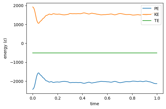
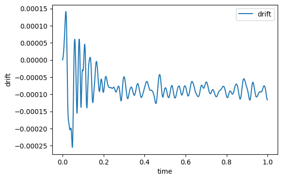
The drift is output to assess the stability of the explicit integration. As a rule of thumb, we would like to keep the drift to below 0.01% of the total energy. The drift reported by mdlj.c is computed as \begin{equation}\label {eq:md:edrift} \Delta \mathscr {T}\left (t\right ) = \frac {\mathscr {T}\left (t\right )-\mathscr {T}\left (0\right )}{\mathscr {T}\left (0\right )} \end{equation} where \(\mathscr {T}\) is the total energy. The plots below show the output trace for the full 1,000 time-steps. We note that with this time-step value (0.001) keeps the total energy conserved to about one part in 10\(^4\).
Now, this invocation of mdlj.c produces an XYZ-format trajectory file (just like mclj did). Here, I have
expanded my XYZ-format convention to allow inclusion of velocities in the output file. Inclusion of velocities is
signified by a 1 on the same line as the number of particles (the first line in each frame). If there is a
1 in that position, then each particle line includes three position coordinates and three velocity
components:
$ more traj.xyz
512 1
BOX 8.44534 8.44534 8.44534
16   0.527833   0.527833   0.527833  -0.982352  -0.823300  -1.530590
16   1.583500   0.527833   0.527833  -0.549726  -0.942381   1.363996
16   2.639167   0.527833   0.527833   1.145014  -0.616762  -1.172725
16   3.694834   0.527833   0.527833   1.520337   3.057595  -1.522653
16   4.750501   0.527833   0.527833  -0.541350  -0.144665  -0.919845
16   5.806168   0.527833   0.527833  -0.221483   1.143893  -1.015784
16   6.861835   0.527833   0.527833   5.752205  -1.045603   1.066189
16   7.917502   0.527833   0.527833   0.819532   0.167275  -1.230297
16   0.527833   1.583500   0.527833  -1.062591   2.169692  -1.318921
16   1.583500   1.583500   0.527833  -1.394993   0.055193   1.411530
...
The number “16” at the beginning designates the “type” as an atomic number; for simplicity, I have decided to
call all of my particles sulfur. (XYZ format is often used for atomically-specific configurations.) The functions
xyz_out() and xyz_in() write and read this format, respectively, in mdlj.c. We will use these functions in
other programs as well, typically those which analyze configuration data. Examples of such analysis codes are
the subjects of the next two sections.
At this point, you can’t do much with all this data, except appreciate just how much data an MD code can produce. In this example, we generated 100 frames of configuration data (positions and velocities) for a 512-atoms system, and the resulting trajectory file is about 3.5 megabytes in size. Of course, that file size scales with both the number of particles and the number of frames it contains. It is not unusual nowadays for researchers to use MD to produce hundreds of gigabytes of configuration data in order to write a single paper. It leads one to think that perhaps a lesson on handling large amounts of data is appropriate for a course on Molecular Simulation; however, I’ll forego that for now by trying to keep our sample exercises small.
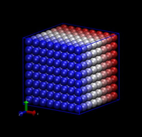
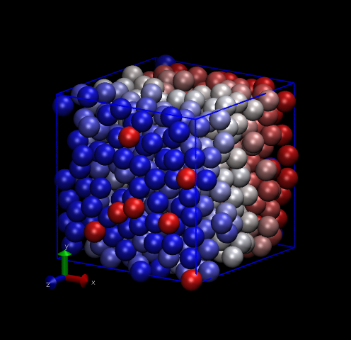
One thing we can do with this data is make nice pictures using VMD. Below are two renderings, one of the initial snapshot, and the other at time \(t\) = 1 (1000 time steps). Notice how the initially perfect crystalline lattice has been wiped out.