9.1 Gromacs
The Gromacs source code is available officially from www.gromacs.org, though some Linux distributions offer pre-compiled versions. In most high-performance computing settings, Gromacs is compiled from source code in order to link in hardware-specific libraries for things like internode communication and compiler-specific math libraries. For this introductory survey though, we can just run the precompiled version on a laptop. (If you have macOS, you might have to compile Gromacs from source.) In Ubuntu under WSL:
$ sudo apt install gromacs
Gromacs is a suite of tools that include an MD engine along with tools for system preparation and simulation analysis. All tools are invoked using the pre-command ‘gmx‘. ‘gmx -help‘ will give a lot of information.
Before proceeding with a couple of practical examples, I must convey the importance of reading the documentation if you want to use Gromacs in your own research. The official Gromacs documentation is extensive, but accessible to beginners. The official tutorials by Justin Lemkul are also a must if you want to learn how to use Gromacs.
Like any MD simulation, using Gromacs breaks down into three main steps:
- 1.
- Prepare system.
- (a)
- Get relevant atomic coordinates;
- (b)
- Decide on a force-field and set the topology;
- (c)
- Add solvent, ions, other atoms as necessary;
- (d)
- Minimize the potential energy.
- 2.
- Run MD.
- 3.
- Analyze results.
As may be inferred, the first step is often the most difficult. It usually requires a lot of care and thought to generate an initial condition for MD. Here we’ll consider just two test cases for which this is not so difficult, but which illustrate the workflow.
9.1.1 A Box of Water
Here I illustrate a workflow for generating and simulating a small box of water molecules.
First, we can use ‘gmx insert-molecules‘ to generate a system with waters randomly positioned inside a box:
$ gmx insert-molecules -ci /usr/share/gromacs/top/spc216.gro \
  -nmol 100 -box 3 3 3 -o water_box.gro
The -box switch allows us to specify a box that is 3x3x3 nm\(^3\), and -ci refers to a special file containing
template atomic coordinates for a single water molecule. The -nmol switch asks Gromacs to try to insert more
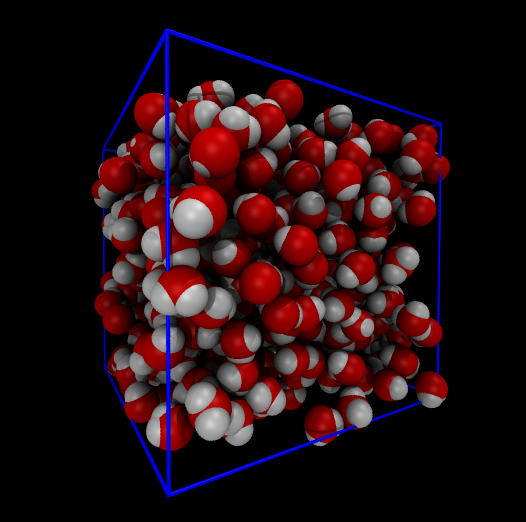
molecules than a simple volume/density calculation would suggest (not many more can be put in). This creates
the file water_box.gro, which for me contains 432 water molecules, as depicted using VMD in
Fig. 32.
Next, we need to use pdb2gmx to generate the Gromacs topology file.
$ gmx pdb2gmx -f water_box.gro -o new_water_box.gro -p topol.top
In running this command, I selected the CHARMM27 force field (which won’t matter since we have nothing but water here) and the TIP3P water model. We now have the topology file and a new gromacs coordinate file (which just renames the water molecules to HOH to conform to the TIP3P naming scheme).
Now, using the minim.mdp parameter file given, we can build and run the energy minimization:
$ gmx grompp -f minim.mdp -c new_water_box.gro -p topol.top -o min.tpr
$ gmx mdrun -v -deffnm min
This will create a lot of output files that all begin with min. One of them contains all the energy-like data:
min.edr. This file is binary, so the tool gmx energy is used to extract data from it:
$ gmx energy -f min.edr
This will create energy.xvg with column-oriented time-series of whatever data is selected interactively.
Fig. 33 shows what the potential energy looks like for this minimization.
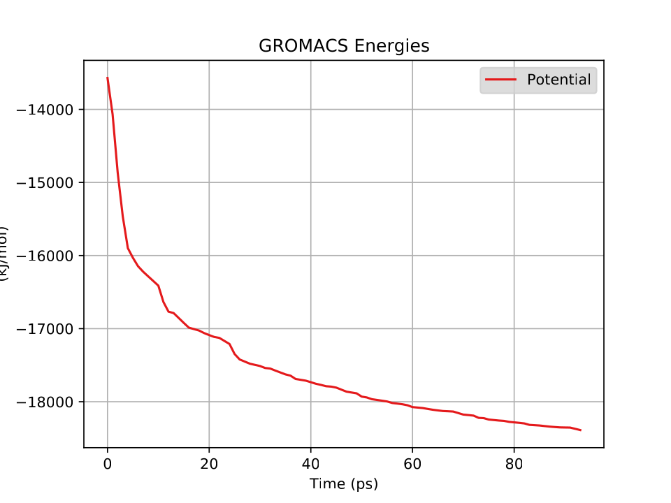
(This is a very, very minimized system; the initial water box had no overlaps really at all.) Now we can run
the NVT simulation using the nvt.mdp parameter file:
$ gmx grompp -f nvt.mdp -c min.gro -p topol.top -o nvt.tpr
$ gmx mdrun -v -deffnm nvt
Fig. 34 shows a plot of the energies vs time for this short, short simulation.
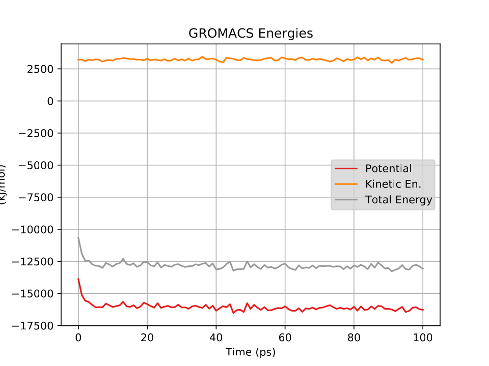
Now let’s try using the output configuration from this NVT simulation as an input for an NPT simulation.
$ gmx grompp -f npt.mdp -c nvt.gro -t nvt.cpt -p topol.top -o npt.tpr
$ gmx mdrun -v -deffnm npt
Fig. 35 shows a plot of the density vs time for this short, short simulation.
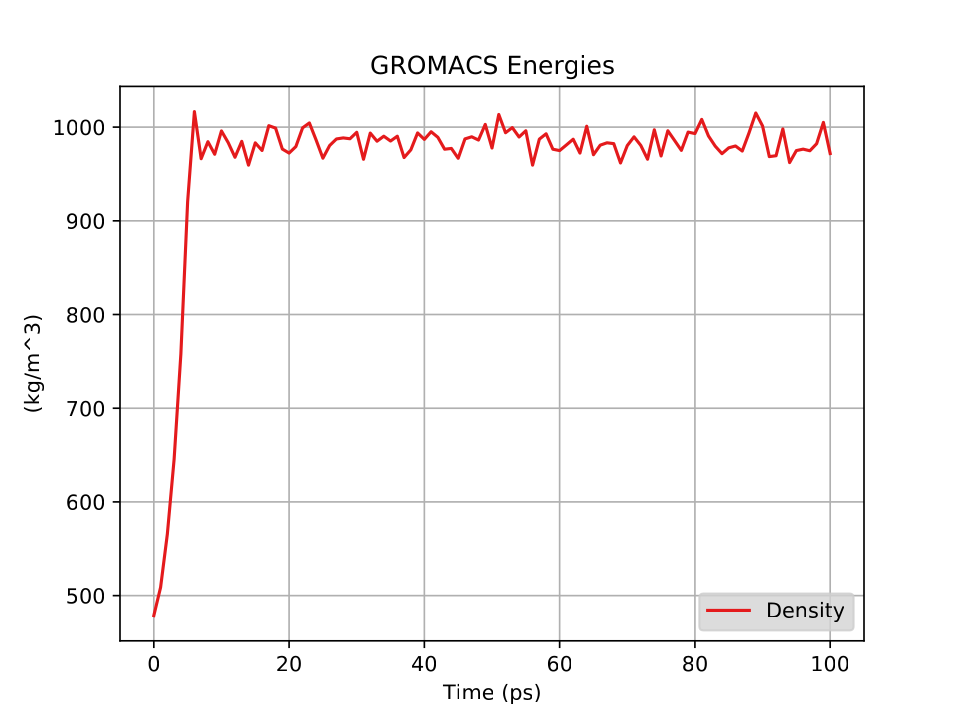
9.1.2 The SARS-CoV-2 spike protein receptor binding domain (RBD)
As a quick example of how to build a protein simulation system, we can consider a very recent example from the Protein Data Bank. The SARS-CoV-2 spike glycoprotein complex is an enormous protein, but a really important part of it are the domains that bind to the ACE2 receptors on the surfaces of epithelial cells. These are called Receptor Binding Domains (RBDs). A lot of recent structural biology has gone into understanding the details of the RBD-ACE2 interface. As an example, take a look at the PDB entry 7c8j, which is the X-ray crystallographic structure of a recombinant construct of the SARS-CoV-2 RBD and the ACE2 ectodomain of the bat [41]. We can use simulations to answer a lot of interesting questions about this structure, but let’s just use it now as a source of coordinates to run a simulation of just the RBD alone.
The first thing to do is to download the PDB file for this entry; there are several ways to do this, but I like to use an interactive VMD session and just put 7c8j in the new molecule file browser. Once VMD has it loaded, the following TcL command in the terminal will create the stripped-down PDB file for just the RBD:
[atomselect top "chain B"] writepdb my_7c8j.pdb
Now we can pretty much follow Justin Lemkul’s lysozyme tutorial here:
# generate the topology; use OPLS-AA force field (sel. 15)
$ gmx pdb2gmx -f my_7c8j.pdb -o my_7c8j_processed.pdb -water spce
# enlarge box
$ gmx editconf -f my_7c8j_processed.pdb -o my_7c8j_newbox.gro \
  -c -d 1.0 -bt cubic
# solvate
$ gmx solvate -cp my_7c8j_newbox.gro
# copy JK’s ions.mdp; add ions (replace group 13)
$ gmx grompp -f ions.mdp -c my_7c8j_solv.gro -p topol.top \
  -o ions.tpr
$ gmx genion -s ions.tpr -o my_7c8j_solv.gro -p topol.top \
  -pname NA -nname CL -neutral
# minimize potential energy using JK’s minim.mdp
$ gmx grompp -f minim.mdp -c my_7c8j_solv.gro -p topol.top -o em.tpr
$ gmx mdrun -v -deffnm em
# have a look at the potential energy
$ gmx energy -f em.edr -o potential.xvg
# copy JK’s nvt.mdp; run NVT MD for 50,000 steps -- this will take a few hours...
$ gmx grompp -f nvt.mdp -c em.gro -r em.gro -p topol.top -o nvt.tpr
$ gmx mdrun -v -deffnm nvt
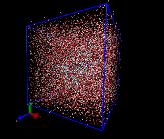
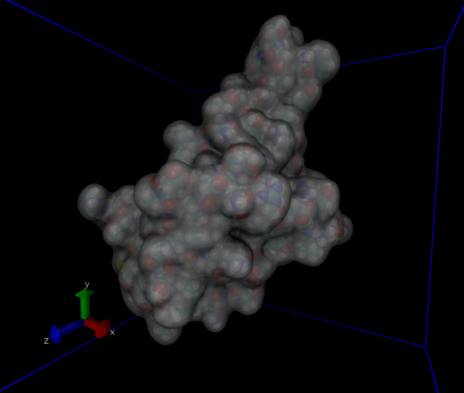
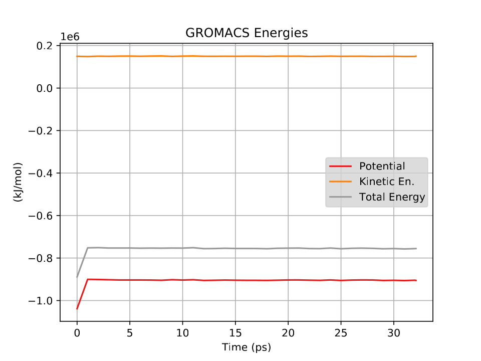
This system has about 60,000 atoms. I show a couple of views from VMD in Fig. 36. For such a large system, we won’t be able to run very long on a laptop; 100 ps takes about 3 hours on mine. Note that we’d typically want to simulate for hundreds of nanoseconds, which would be several thousand hours on my laptop, or a a day or so on a supercomputer. After about 30 ps (an hour), I went ahead and made a plot of the energies (Fig. 37).