5.3 Case Study 2: Static Properties of the Lennard-Jones Fluid
5.3.1 Running the code
The code mdlj.c was run on 108 particles with positions initialized on a simple cubic lattice at a density \(\rho \) = 0.8442 and temperature (specified by velocity assignment and scaling) initially set at \(T\) = 0.728. A single run of 600,000 time steps was performed, which took about 2 minutes on my laptop. (This is almost 10\(^6\) particle-updates per second; not bad for a laptop running a silly \(N^2\) pair search, but it’s only for \(\sim \) 100 particles...the same algorithm applied to 10,000 would be slower.) The commands I issued looked like:
$ mkdir md_cs2
$ cd md_cs2
$ ../mdlj -N 108 -fs 1000 -ns 600000 -rho 0.8442 -T0 0.728 -rc 2.5 -traj traj1.xyz -prog 100 >& 1.out &
$ tail -f 1.out
468900 468.90000 -475.45590 242.36056 -233.09534 -2.79034e-04 1.49605 5.43064
469000 469.00000 -475.67663 242.58353 -233.09310 -2.88639e-04 1.49743 5.11914
469100 469.10000 -477.58731 244.49557 -233.09175 -2.94452e-04 1.50923 4.88396
469200 469.20000 -457.41152 224.32176 -233.08975 -3.02989e-04 1.38470 5.82717
469300 469.30000 -492.03036 258.93556 -233.09481 -2.81326e-04 1.59837 4.82093
469400 469.40000 -465.44072 232.34350 -233.09723 -2.70947e-04 1.43422 5.69688
469500 469.50000 -478.52166 245.42514 -233.09652 -2.73957e-04 1.51497 5.01491
469600 469.60000 -469.00769 235.90985 -233.09784 -2.68307e-04 1.45623 5.64466
469700 469.70000 -476.27992 243.18354 -233.09637 -2.74603e-04 1.50113 5.34172
469800 469.80000 -461.91910 228.82734 -233.09176 -2.94382e-04 1.41251 5.68907
469900 469.90000 -469.00227 235.90429 -233.09798 -2.677^C
The final \& puts the simulation “in the background,” and returns the shell prompt to you. The tail -f
command allows you to “watch” as the log file is written to. You can also verify that the job is running by issuing
the “top” command, which displays in the terminal the a listing of processes using CPU, ranked by how
intensively they are using the CPU. This command “takes over” your terminal to display continually updated
information, until you hit Ctrl-C.
top - 13:43:27 up 4 days,  6:19,  0 users,  load average: 0.16, 0.45, 0.28
Tasks:  29 total,   2 running,  27 sleeping,   0 stopped,   0 zombie
%Cpu(s): 12.7 us,  0.0 sy,  0.0 ni, 83.3 id,  0.0 wa,  0.0 hi,  4.0 si,  0.0 st
MiB Mem :  12608.9 total,  11169.1 free,    739.2 used,    700.7 buff/cache
MiB Swap:   4096.0 total,   4096.0 free,      0.0 used.  11616.8 avail Mem

  PID USER      PR  NI    VIRT    RES    SHR S  %CPU  %MEM     TIME+ COMMAND
14668 cfa       20   0    6652   1268   1116 R 100.0   0.0   0:02.83 mdlj
13073 cfa       20   0  863448  47256  28728 S   6.7   0.4   0:19.24 node
    1 root      20   0    1020    648    520 S   0.0   0.0   1:29.57 init
    8 root      20   0     888     76     16 S   0.0   0.0   0:00.00 init
    9 root      20   0     888     76     16 S   0.0   0.0   1:04.20 init
   10 cfa       20   0   10164   4980   3188 S   0.0   0.0   0:00.11 bash
  168 root      20   0     984    172     16 S   0.0   0.0   0:00.00 init
From the command line arguments shown above, we can see that this simulation run will produce 601
snapshots, beginning with \(t=0\) and outputting every 1000 steps. Each frame has 108 lines of 69 bytes each, plus
another 30 for the header in each frame, so basically every frame is 7,482 bytes. With 601 of them, that is
4,496,682 bytes, or 4.2884 megabytes (1 megabyte is 1,048,576 bytes). We can confirm this calculation using
the du (disk usage) command:
$ du -sh traj1.xyz
4.3M    traj1.xyz
Thirty years ago, one might have raised an eyebrow at this; nowadays, this is very nearly an insignificant amount of storage.
5.3.2 Equilibration and Decorrelation
An important purpose of this case study is to quantify the notion of “equilibration” of the system by assessing correlations in (apparently) randomly fluctuating quantities like potential energy. Remember, in order to perform accurate ensemble averaging over an MD trajectory, we have to be sure that correlations in the properties we are measuring have “died out.” This is another way of saying that the length of the time interval over which we conduct the time average must be much longer than the correlation time. In this case study, we illustrate the “block averaging” technique of Flyvbjerg and Petersen [7] to determine the equilibration time-scale of the potential energy.
First, compute the variance of the \(L\) samples of \(\mathscr {U}\): \begin{equation} \sigma ^2_0\left ({\mathscr {U}}\right ) \approx \frac {1}{L}\sum _{i=1}^{L}\left [\mathscr {U}_i - \bar {\mathscr {U}}\right ]^2 \end{equation} This is approximate because of so far undetermined
time-correlations in \(\mathscr {U}\); that is, not all \(L\) samples are uncorrelated. For example, two samples one time-step apart
will likely be very close to one another. Now, we block the data by averaging \(L/2\) pairs of adjacent values: \begin{equation} \mathscr {U}_i^{(1)} = \frac {\mathscr {U}_{2i-1} + \mathscr {U}_{2i}}{2} \end{equation} The \((1)\)
superscript indicates that this is a “first-generation” coarsening of the potential energy trace. The variance of
this new set, \(\sigma ^2_1\) is computed. Then the process is recursively carried out through many subsequent
generations. After many blocking operations, the coarsened samples, \(\mathscr {U}_i^{(j)}\), become uncorrelated, and the
variance saturates (temporarily). This means we should observe a plateau in a plot of variance vs
generation. The Python program flyvberg.py implements this calculation using outputs of mdlj.c as
inputs.
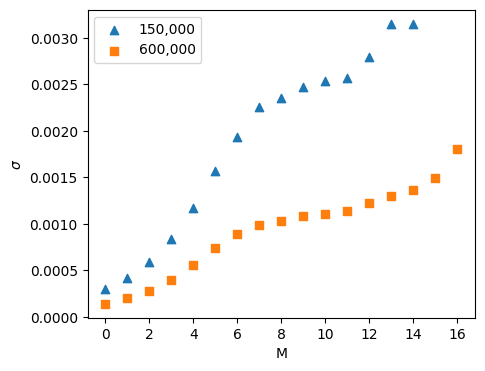
According to the discussion of this blocking technique, the standard deviation shows a dependence on the blocking degree, \(M\), when the blocked averages are correlated, and plateaus at a blocking degree for which the averages become uncorrelated. This blocking degree corresponds to a time interval of length \(2^M\). This data indicates that potential energy decorrelates after a time of approximately \(2^{10} \approx 1000\) steps. This is a reassuring result, as we could have guessed that 1000 steps are required based on the initial transience in the energy traces seen in the previous figure. I ran three independent simulations, each differing only in the random number seed used. The results are shown in Table 1.
| Run | \(\left <\mathscr {U}\right >/N\) | \(\left <\mathscr {K}\right >/N\) | \(\left <\mathscr {T}\right >\) | \(\left <P\right >\) |
| 1 | \(-4.4165 \pm 0.0012\) | \(2.2577 \pm 0.0012\) | \(1.5051 \pm 0.0008\) | \(5.1960 \pm 0.0057\) |
| 2 | \(-4.4188 \pm 0.0010\) | \(2.2597 \pm 0.0010\) | \(1.5064 \pm 0.0007\) | \(5.1948 \pm 0.0050\) |
| 3 | \(-4.4157 \pm 0.0011\) | \(2.2564 \pm 0.0011\) | \(1.5043 \pm 0.0008\) | \(5.2022 \pm 0.0055\) |
| Avg. | \(-4.4170 \pm 0.0011\) | \(2.2579 \pm 0.0011\) | \(1.5053 \pm 0.0008\) | \(5.1977 \pm 0.0054\) |
5.3.3 Radial Distribution Functions and Postprocessing
A second major objective of this case study is to demonstrate how to compute the radial distribution function, \(g(r)\). The radial distribution function is an important statistical mechanical function that captures the structure of liquids and amorphous solids. We can express \(g(r)\) using the following statement: \begin{equation} \rho g(r) = \text {average density of particles at } {\bf r} \text { given that a tagged particle is at the origin} \end{equation}
The procedure we will follow will be to write a second program (a “postprocessing code”) which will read in the trajectory output produced by the simulation, mdlj.c. The general structure of a \(g(r)\) post-processing code could look like this:
- 1.
- Determine trajectory time limits: start, stop, and step
- 2.
- Initialize histogram.
- 3.
- Read in the trajectory as a list of frames.
- 4.
- For each frame:
- (a)
- Visit all unique pairs of particles, and update histogram for each visit if applicable
- 5.
- Normalize histogram and output.
- 6.
- End.
We will consider a code, rdf.c, that implements this algorithm for computing \(g(r)\), but first we
present a brief argument for post-processing vs on-the-fly processing for computing quantities such
as \(g(r)\). For demonstration purposes, it is arguably simpler to drop in a \(g(r)\)-histogram update sampling
function into an existing MD simulation program to enable computation of \(g(r)\) during a simulation,
compared to writing a wholly separate program. After all, it nominally involves less coding. The
counterargument is that, once you have a working (and eventually optimized) MD simulation code,
one should be wary of modifying it. The purpose of the MD simulation is to produce samples.
One can produce samples once, and use any number of post-processing codes to extract useful
information. The counterargument becomes stronger when one considers that, for particularly
large-scale simulations, it is simply not convenient to re-run an entire simulation when one discovers a
slight bug in the sampling routines. The price one pays is that one needs the disk space to store
configurations.
As shown earlier, one MD simulation of 108 particles out to 600,000 time steps, storing configurations every 1,000 time steps, requires less than 5 MB. This is an insignificant price. Given that we know that the MD simulation works correctly, it is sensible to leave it alone and write a quick, simple post-processing code to read in these samples and compute \(g(r)\).
The code rdf.c is a C-code implementation of just such a post-processing code. This program illustrates a
different way to abstractify the trajectory, namely as a list of frames. A frame is an instance of an abstract data
type called frametype that we define (for now) in rdf.c, along with a special function NewFrame() to
allocate memory for a frame, and another read_xyz_frame() to read a frame in from an XYZ-format
trajectory:
typedef struct FRAME {
    double * rx, * ry, * rz;  // coordinates
    double * vx, * vy, * vz;  // velocities
    int * typ; // array of particle types 0, 1, ...
    int N; // number of particles
    double Lx, Ly, Lz; // box dimensions
} frametype;

/* Create and return an empty frame */
frametype * NewFrame ( int N, int hv ) {
    frametype * f = (frametype*)malloc(sizeof(frametype));
    f->N=N;
    f->rx=(double*)malloc(sizeof(double)*N);
    f->ry=(double*)malloc(sizeof(double)*N);
    f->rz=(double*)malloc(sizeof(double)*N);
    if (hv) {
        // caller has requested a frame with space for velocities
        f->vx=(double*)malloc(sizeof(double)*N);
        f->vy=(double*)malloc(sizeof(double)*N);
        f->vz=(double*)malloc(sizeof(double)*N);
    } else {
        f->vz=NULL;
        f->vy=NULL;
        f->vx=NULL;
    }
    f->typ=(int*)malloc(sizeof(int)*N);
    return f;
}
/* Read an XYZ-format frame from stream fp; returns the new frame.
   Note the non-conventional use of the first line to indicate
   whether or not the frame contains velocities and the comment
   line to hold boxsize information. */
frametype * read_xyz_frame ( FILE * fp ) {
    int N,i,j,hasvel=0;
    double x, y, z, Lx, Ly, Lz, vx, vy, vz;
    char typ[3], dummy[5];
    char ln[255];
    frametype * f = NULL;
    if (fgets(ln,255,fp)){
        sscanf(ln,"%i %i\n",&N,&hasvel);
        f = NewFrame(N,hasvel);
        fgets(ln,255,fp);
        sscanf(ln,"%s %lf %lf %lf\n",dummy,&f->Lx,&f->Ly,&f->Lz);


        for (i=0;i<N;i++) {
            fgets(ln,255,fp);
            sscanf(ln,"%s %lf %lf %lf %lf %lf %lf\n",
                   typ,&f->rx[i],&f->ry[i],&f->rz[i],&vx,&vy,&vz);
            if (hasvel) {
                f->vx[i]=vx;
                f->vy[i]=vy;
                f->vz[i]=vz;
            }
            j=0;
            while(strcmp(elem[j],"NULL")&&strcmp(elem[j],typ)) j++;
            if (strcmp(elem[j],"NULL")) f->typ[i]=j;
            else f->typ[i]=-1;
        }
    }
    return f;
}
With this abstract data type, we no longer need to pass all parallel arrays as separate parameters; we can
instead just pass a pointer frametype*. For example, below is the function rij that computes the
minimum-image convention distance between particles i and j in a particular frame:
/* Compute scalar distance between particles i and j in frame f;
   note the use of the minimum image convention */
double rij ( frametype * f, int i, int j ) {
    double dx, dy, dz;
    double hLx=0.5*f->Lx,hLy=0.5*f->Ly,hLz=0.5*f->Lz;
    dx=f->rx[i]-f->rx[j];
    dy=f->ry[i]-f->ry[j];
    dz=f->rz[i]-f->rz[j];
    if (dx<-hLx) dx+=f->Lx;
    if (dx> hLx) dx-=f->Lx;
    if (dy<-hLy) dy+=f->Ly;
    if (dy> hLy) dy-=f->Ly;
    if (dz<-hLz) dz+=f->Lz;
    if (dz> hLz) dz-=f->Lz;
    return sqrt(dx*dx+dy*dy+dz*dz);
}
Using rij() it is then easy to update the RDF histogram:
/* An N^2 algorithm for computing interparticle separations
   and updating the radial distribution function histogram. */
void update_hist ( frametype * f, double rcut,
                   double dr, int * H, int nbins ) {
    int i,j;
    double r;
    int bin;
    for (i=0;i<f->N-1;i++) {
        for (j=i+1;j<f->N;j++) {
            r=rij(f,i,j);
            if (r<rcut) {
                bin=(int)(r/dr);
                if (bin<0||bin>=nbins) {
                    fprintf(stderr,
                            "Warning: %.3lf not on [0.0,%.3lf]\n",
                            r,rcut);
                } else {
                    H[bin]+=2;
                }
            }
        }
    }
}
H is the histogram. One can see that the bin value is computed by first dividing the actual distance between
members of the pair by the resolution of the histogram, \(\delta r\), and casting the result as an integer. This resolution
can be specified on the command-line when rdf.c is executed. Also notice that the histogram is updated by 2,
which reflects the fact that either of the two particles in the pair can be placed at the origin. Also notice the
implementation of the minimum image convention.
In the main() function of rdf.c, a simple block of code can read in a whole trajectory from a file named by
trajfile and store it in an array of frametype* pointers:
    i=0;
    fprintf(stdout,"Reading %s\n",trajfile);
    fp=fopen(trajfile,"r");
    while (Traj[i++]=read_xyz_frame(fp));
    nFrames=i-1;
    fclose(fp);
    if (!nFrames) {
        fprintf(stdout,"Error: %s has no data.\n",trajfile);
        exit(-1);
    }
    fprintf(stdout,"Read %i frames from %s.\n",nFrames,trajfile);
Then a second block of code allocates, initializes, and computes the pair correlation histogram:
    /* Adjust cutoff and compute histogram */
    L2min=min(Traj[0]->Lx/2,min(Traj[0]->Ly/2,Traj[0]->Lz/2));
    if (rcut>L2min) rcut=L2min;
    nbins=(int)(rcut/dr)+1;
    H=(int*)malloc(sizeof(int)*nbins);
    for (i=0;i<nbins;i++) H[i]=0;
    for (i=begin_frame;i<nFrames;i++)
        update_hist(Traj[i],rcut,dr,H,nbins);
    nFramesAnalyzed=nFrames-begin_frame;
Note that the cutoff rcut may not exceed half a box length in any dimension. The number of histogram bins is
simply one plus the cutoff divided by the resolution dr. The variable begin_frame allows the caller to gather
statistics only after a certain number of frames in the trajectory in order to “ignore” initial frames where the initial
configuration is still “remembered”.
Finally, once the trajectory has been traversed and the histrogram computed, it is then normalized by compute \(g(r)\) and save the result to a designated output file:
    /* Normalize and output g(r) to the terminal */
    /* Compute density, assuming NVT ensemble */
    fp=fopen(outfile,"w");
    fprintf(fp,"# RDF from %s\n",trajfile);
    fprintf(fp,"#LABEL r g(r)\n");
    fprintf(fp,"#UNITS %s *\n",length_units);
    /* Ideal-gas global density; assumes V is constant */
    rho=Traj[0]->N/(Traj[0]->Lx*Traj[0]->Ly*Traj[0]->Lz);
    for (i=0;i<nbins-1;i++) {
        /* bin volume */
        vb=4./3.*M_PI*((i+1)*(i+1)*(i+1)-i*i*i)*dr*dr*dr;
        /* number of particles in this shell if this were
           an ideal gas */
        nid=vb*rho;
        fprintf(fp,"%.5lf %.5lf\n",i*dr,
                (double)(H[i])/(nFramesAnalyzed*Traj[0]->N*nid));
    }
    fclose(fp);
    fprintf(stdout,"%s created.\n",outfile);
(The variable length_units is a string that just labels the length units; by default, this is "sigma", indicating LJ
\(\sigma \).)
Now, let’s execute rdf from one of our 600,000-time-step simulations’ 6,001-frame trajectory, ignoring the
first 1,000 frames (100,000 time steps):
$ cd ~/dxu/chet580/instructional-codes/my_work/mdlj/set1
$ gcc -O5 -o rdf ../../../originals/rdf.c -lm
$ ./rdf -t traj-rho0.90-rep0.xyz -dr 0.02 -rcut 3.5 \
   -o rdf-rho0.90-rep0.dat -begin-frame 1000
Reading traj-rho0.90-rep0.xyz
Read 6001 frames from traj-rho0.90-rep0.xyz.
rdf-rho0.90-rep0.dat created.
$
Using the python program plot_rdf.py, we can generate a plot of this RDF (Fig. 17:
$ python ../../../originals/plot_rdf.py -i rdf-rho0.90-rep0.dat \
  -o rdf-rho0.90-rep0.png
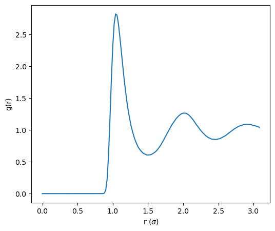
This \(g(r)\) shows a peak at about 2\(^{1/6}\sigma \) that corresponds to the LJ well, indicating that there is a dense
nearest-neighbor shell out to about 1.5 \(\sigma \). How dense? We can use \(g(r)\) to count particles within a
distance \(r\) from a central atom: \begin{equation} \label {eq:md:ungr} n\left (r\right ) = \rho \int _0^r\int _0^{\pi }\int _0^{2\pi } g\left (r^\prime \right ) \left (r^\prime \right )^2\sin \theta dr^\prime d\theta d\phi = 4\pi \rho \int _0^r \left (r^\prime \right )^2g\left (r^\prime \right )dr^\prime \end{equation} This integration is enabled in plot_rdf.py via the -rho and -R
flags:
$ python ../../../originals/plot_rdf.py -i rdf-rho0.90-rep0.dat \
  -o rdf-rho0.90-rep0.png -rho 0.9 -R 1.5
n=12.335
This indicates the nearest neighbor shell is pretty well packed; spherical close-packing would be exactly 12.