4.4 Case Study 2: MC of Hard Disks
Change directory into your instructional-codes repository and issue a pull if you don’t already see hdisk.c
there. This code simulates disks confined to a circle. The Hamiltonian for this system may be expressed as \begin{equation} \mathscr {H} = \sum _{i=1}^N H_1({\bf r}_i) + \sum _{i=1}^{N}\sum _{j=i+1}^{N} H_2({\bf r}_i,{\bf r}_j) \end{equation}
where \begin{equation} H_1({\bf r}_i) = \left \{\begin {array}{ll} 0 & r_i < R\\ \infty & r_i > R \end {array}\right . \end{equation} and \begin{equation} H_2({\bf r}_i,{\bf r}_j) = \left \{\begin {array}{ll} 0 & \sqrt {\left ({\bf r}_i-{\bf r}_j\right )^2} > \sigma \\ \infty & \sqrt {\left ({\bf r}_i-{\bf r}_j\right )^2} < \sigma \end {array}\right . \end{equation}
\(H_1\) acts to keep the particles confined, and \(H_2\) prevents them from overlapping. One nice thing about using hard-disk Hamiltonians is that there is never a reason to evaluate a Boltzmann factor. Any trial move that results in an overlap or a particle crossing the boundary gives an “infinite” \(\Delta {U}\), so \(e^{-\beta \Delta {U}}\) is identically 0 and the trial is unconditionally rejected.
hdisk.c requires as user input any two of the following three parameters: \(R\), the radius of the circle in \(\sigma \); \(\rho \), the
areal number density of particles (# per square \(\sigma \)); and \(N\), the number of particles. The user may also specify \(\delta r\), the
scalar displacement, and nc, the number of MC cycles, where one cycle is \(N\) attempted particle displacements.
Optionally, the code can generate configurational samples as simple text files or as a single XYZ-formatted
trajectory (which looks like a concatenation of XYZ files), and in order to generate these samples,
traj_samp must be set greater than zero. The code reports the acceptance ratio, among other things:
\[ \left [\begin {array}{c} \mbox {acceptance}\\ \mbox {ratio} \end {array}\right ] = \left [\frac {\mbox {number of successful trials}}{\mbox {number of trials}}\right ] \]
One important aspect of any MC simulation code is how the particle positions are initialized. Here, it is best
to assign initial positions to the particles such that the initial energy is 0 (i.e., there are no overlaps nor particles
out of bounds.) Try to figure out how the function init() in the program hdisk.c accomplishes
this.
As a suggested further exercise, use hdisk.c to determine a reasonable displacement to achieve a 30%
acceptance ratio at a density of 0.5. Compare your results across differently sized systems and runs with
different numbers of cycles. For fewer than 10\(^6\) cycles, you will have large acceptance ratios because the initial
condition is not yet fully destroyed.
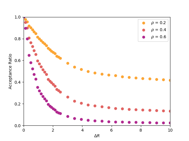
Below is a plot of acceptance ratio vs. \(\Delta R\) for densities \(\rho \) of 0.2, 0.4, 0.6, from a simulations of 200 particles. 2,000 cycles were performed for each run, and each had a unique seed. Are your results consistent with this data?
One advantage of the XYZ format is that we can use VMD to visualize our configurations, and even to make animations of our simulations. For example, suppose we generate a short 1,000-cycle MC trajectory of the hard-disk system at \(\rho \) = 0.7 and \(N\) = 100:
cd
cd cheT580-202035/instructional-codes/my_work
mkdir hdisk_run
cd hdisk_run
gcc -O3 -o hdisk ../../originals/hdisk.c -lm -lgsl
./hdisk -xyz traj.xyz -traj_samp 1 -nc 1000 -rho 0.7 -N 100 -dr 0.5
# R = 6.74336; rho = 0.70000; N = 100; seed = 23410981
Results:
Number of Trial Moves:          100000
Maximum Displacement Length:    0.50000
Acceptance Ratio:               0.48499
Reject Fraction Out-of-bounds:  0.09707
Reject Fraction Overlap:        0.90293
ls
hdisk traj.xyz
Notice I provide the name of the trajectory file, indicating I want one sample per cycle. I also set the magnitude of the maximum displacement at 0.5 \(\sigma \).
After the run finishes, the file traj.xyz appears. It looks like this:
head -10 traj.xyz
100
Generated by hdisk.c; all z-components are zero; all elements are H
H 2.48776 1.78242 0.00000
H 5.80283 0.16579 0.00000
H 2.57789 -4.28715 0.00000
H -4.25852 0.68353 0.00000
H -5.95301 2.69712 0.00000
H 0.28903 -1.04400 0.00000
H 1.86426 -0.93249 0.00000
H -4.16984 1.87756 0.00000
We can use VMD to visualize this trajectory. If you are on a Windows 10 machine and you installed the Windows version of VMD, you can simply launch it from the start menu, and then navigate to
\\wsl\$\<distro>\home\<username>\cheT580-202035\instructional-codes\my_work\hdisk_run\
and then just click on traj.xyz to read it in. If you are on a Mac, you should be able to navigate
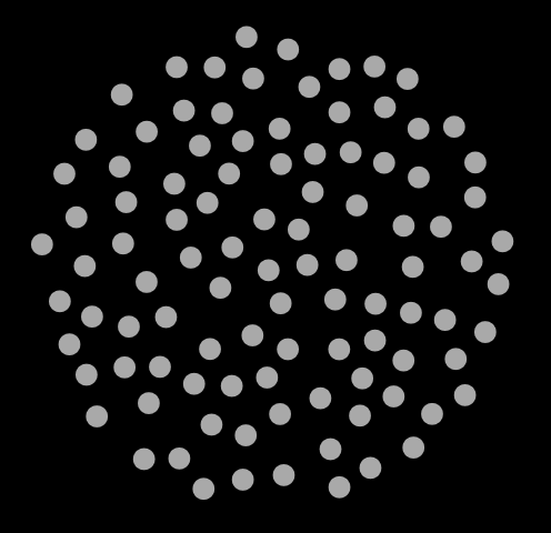
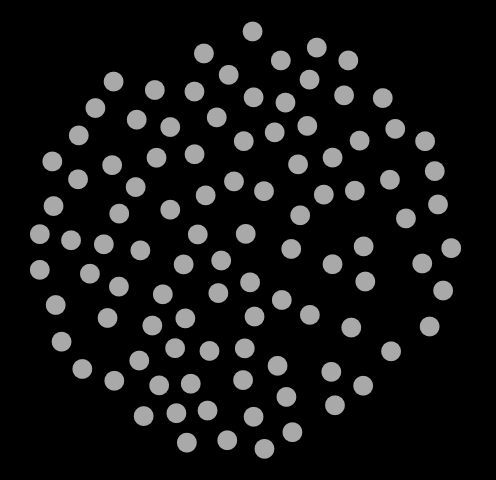
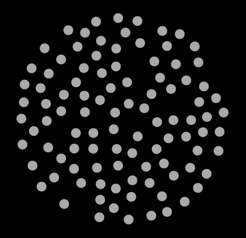
straight to the file. In Fig. 7, I show three snapshots from this simulation, at cycle 0, 500, and
1000.
As another suggested exercise, consider generating a trial move in the following way:
- 1.
- Randomly select a particle \(i\).
- 2.
- Randomly choose a direction. In 2D, this is an angle \(\phi \) chosen uniformly from the interval \([0,2\pi ]\). In 3D, this is two angles \(\theta \) and \(\phi \), where \(\cos \theta \) is chosen uniformly from the interval \([-1,1]\), and \(\phi \) is chosen uniformly from the interval \([0,2\pi ]\).
- 3.
- Compute the displacement vector components. In 2D: \(dx = \Delta R\cos \theta \) and \(dy = \Delta R\sin \theta \). In 3D: \(dx = \Delta R\sin \theta \cos \phi \), \(dy = \Delta R\sin \theta \sin \phi \), \(dz = \Delta R\cos \theta \).
- 4.
- Execute the move by adding the displacement vector components to the position of particle \(i\).
The main difference of this scheme with the first one is that, in 2D, only one random number must be chosen per displacement attempt. Explore the acceptance ratio vs. \(\Delta R\) relationship with this new trial move. Does this scheme generate a 30% acceptance ratio for a higher or lower maximum displacement that does the original scheme?