Elements of a Continuous-Space MC program

4.3 Elements of a Continuous-Space MC program

The Ising system serves us well as a simple introduction to the technique of Monte Carlo simulation. Now, we move on to the more advanced case of continuous-space Monte Carlo; that is, Monte Carlo on a system composed of particles whose position and velocity vector components are real numbers. We will first consider the simple case of a “hard-sphere” liquid, and then the more realistic Lennard-Jones liquid. These distinctions have to do with the potential energy function used to compute the potential energy \(U\) of a configuration \({\bf r}^N\).

Regardless of the potential used, all continuous-space MC programs have common elements:

1.: data representation and input/output;
2.: energy calculation;
3.: trial move generation.

4.3.1 Data Representation and Input/Output

The information that must be stored and handled in an MC program are the particle positions. In 3D space, each particle has three components of its position. The simplest way to represent this information in a program is by using parallel arrays; that is, three arrays, dimensioned from 1 to \(N\), one for each dimension. In C, we might declare these arrays for 1,000 particles as

  int N = 1000;
  double rx[N], ry[N], rz[N];

This data can be stored in standard ASCII text files, or in unformatted binary files. In fact, a large part of most molecular simulation is producing and storing configurations which can be processed “offline” (away from the simulation program) to perform analyses. A simple and widely used ASCII configuration file format is called “XYZ”. A code fragment to write a configuration of \(N\) hydrogen atoms in XYZ format appears below:

  FILE * fp;
  ...
  fp = fopen("my_config.xyz","w");
  fprintf(fp,"%i\n",N);
  fprintf(fp,"This is a comment or just a blank line\n");
  for (i=0;i<N;i++)
    fprintf(fp,"%s %.8le %.8le %.8le\n","H",rx[i],ry[i],rz[i]);

The main feature of XYZ files is that one can specify the element type of each atom; for simple visualization purposes of our toy systems, this can be anything, so we’ll just use H for now.

It’s quite easy to read ASCII data in that was written in XYZ format, e.g., using the fragment above, ignoring the element types (for now):

  FILE * fp;
  int N;
  double * rx, * ry, * rz;
  char dummy[4];
  ...
  fp = fopen("my_config.xyz","r");
  fscanf(fp,"%i\n",&N);
  /* allocate if not done already */
  rx=(int*)malloc(N*sizeof(int));
  ry=(int*)malloc(N*sizeof(int));
  rz=(int*)malloc(N*sizeof(int));
  fscanf(fp,"\n"); /* reads the comment line but throws it away */
  for (i=0;i<N;i++)
    fscanf(fp,"%s %.8le %.8le %.8le\n",dummy,&rx[i],&ry[i],&rz[i]);

4.3.2 Analytical Potentials

The total system potential energy is most often computed by means of analytical potentials. Such a potential energy can be written as a continuous function of the positions of particle centers-of-mass. (Such potentials are often termed “empirical” when applied to atomic systems because they formally neglect quantum mechanics.) In most molecular simulations, the total system potential can be decomposed in the following way: \begin{equation} {U}\left ({\bf r}^N\right ) = U_0 + \sum _i U_1( {\bf r}_i ) + \sum _{i<j} U_2( {\bf r}_i, {\bf r}_j ) + \sum _{i<j<k} U_3( {\bf r}_i, {\bf r}_j, {\bf r}_k ) + \cdots + U_N( {\bf r}_i, {\bf r}_j, \dots , {\bf r}_N ), \end{equation} Here, \(U_0\) is some reference potential. \(U_1\) is a “one-body” potential, \(U_2\) is a “two-body” potential, etc. This generally defines a “many-body” potential, and is the heart of the “many-body” problem of statistical physics. Namely, the Boltzmann factor \(e^{-\beta {U}}\) correlates every position with every other position, and the configurational integral (Eq. 47) is not factorizable into many separate easily evaluated integrals.

Analytical potentials are most easily understood by considering model systems which are decomposable into spherically-symmetric, pairwise interactions. Consider then the following total system potential energy: \begin{equation} {U} = \sum _{i=1}^{N}\sum _{j=i+1}^{N} U_{ij}\left (r_{ij}\right ) \end{equation} The double-sum runs over all unique pairs of particles. The function \(U_{ij}\left (r_{ij}\right )\) is called a pair potential, and it is a function of the scalar distance between particle \(i\) and \(j\).

The simplest pair potential is the “hard-sphere”: \begin{equation} \label {eq:hs} U_{HS}\left (r\right ) = \left \{\begin {array}{ll} \infty & r < \sigma \\ 0 & r > \sigma \end {array}\right . \end{equation} Here, \(\sigma \) is an arbitrary interaction range that denotes the “size” of the spheres. When the distance between two spheres is less than \(\sigma \), the energy is infinite; otherwise it is 0. This is the simplest way to enforce excluded volume among spherical particles in an MC simulation. We will see an implementation of a hard-sphere liquid in the next section.

The most celebrated pair potential is the Lennard-Jones potential (Fig. 5): \begin{equation} \label {eq:lj} U_{LJ}\left (r\right ) = 4\epsilon \left [\left (\frac {\sigma }{r}\right )^{12}-\left (\frac {\sigma }{r}\right )^{6}\right ] \end{equation} \(\epsilon \) is the unit of energy, and is the well-depth of the pair potential (that is, it is the minimum value of the potential). \(\sigma \) is the unit of length, and is the separation distance when the potential is identically zero. Unlike the hard-sphere potential (Eq. 76), the Lennard-Jones potential is “smooth” (it has a continuous first derivative). This smoothness makes it useful in Molecular Dynamics simulations, as we will see later in the course.

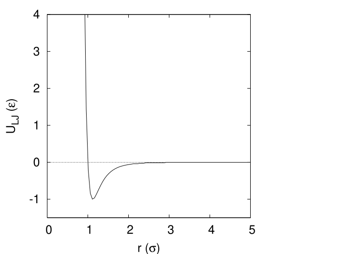
Figure 5: The Lennard-Jones pair potential.

We will encounter more complex potentials than Lennard-Jones, but it serves as a useful tool for introductory molecular simulation.

Reduced Units. Because the Lennard-Jones potential is so prevalent in molecular simulations, it is essential that we understand the unit system most often chosen for simulations using this potential. For computational simplicity, energy in a Lennard-Jones system is measured in units of \(\epsilon \) and length in \(\sigma \). This means that everywhere in the code you would expect to see \(\epsilon \) or \(\sigma \), you find a 1 (often implied).

Now, to compute the total potential \(U\) for a system of particles, the simplest algorithm is to loop over all unique pairs of particles. Here is a simple pair search C function (the so-called \(N^2\) algorithm because its complexity scales like \(N^2\)) to compute the total energy of a system of Lennard-Jones particles, in reduced units:

double total_e ( double * rx, double * ry, double * rz, int n ) {
   int i,j;
   double dx, dy, dz, r2, r6, r12;
   double e = 0.0;
   for (i=0;i<(n-1);i++) {
     for (j=i+1;j<n;j++) {
        dx  = rx[i]-rx[j];
        dy  = ry[i]-ry[j];
        dz  = rz[i]-rz[j];
        r2  = dx*dx + dy*dy + dz*dz;
        r6  = r2*r2*r2;
        r12 = r6*r6;
        e  += 4*(1.0/r12 - 1.0/r6);
     }
   }
   return e;
}

Although it is strictly correct, the \(N^2\) pair search algorithm is inefficient if there is a finite interaction range in the pair potential. Typically in dense liquid simulations, a Lennard-Jones pair potential is truncated at \(r = 2.5\ \sigma \). There are some potentials that are cut off at even shorter distances. The point is that, when the maximum interaction distance is finite, each particle has a finite maximum number of interaction partners. (This assumes number density is bounded, which is a reasonable assumption.) More advanced techniques (which we discuss later) can be invoked to make the pair search much more efficient in this case. The two most common are (1) the Verlet list, and (2) the link-cell list. For now, and to keep the presentation simple, we will stick to the inefficient, brute-force \(N^2\) algorithm.

4.3.3 Trial Moves

Particle Displacement. The most common trial move in continuous-space MC is a particle displacement. First, a small number \(\Delta R\), representing a maximum displacement, is set. A trial move consists of

1.: Randomly select a particle, \(i\).
2.: Displace x-position coordinate of particle \(i\) by a random amount, \(\delta x\), which is given by \begin{equation} \delta x = \Delta R \xi _x \end{equation} where \(\xi _x\) is a uniform random variate on the interval [-0.5:0.5].
3.: Repeat for the \(y\) and \(z\) coordinates, if applicable.

This move guarantees detailed balance, provided that the random particle selection is uniform; for any given move, selection of all possible particles is equally likely. This means that probability of suggesting a move that displaces a particle, going from a state \(n\) to a new state \(m\), has the same probability of selecting the same particle while in state \(m\) and giving it a displacement that will return the configuration to state \(n\). (Do you think such sequential moves ever actually happen?)

For a system of simple particles, random displacements are the only necessary trial moves; thus, \(\alpha _{nm}\) is always unity. For more complicated systems, there are zoos of trial moves all over the literature. We will consider some more complicated systems and trial moves later in the course; one that we consider next is rigid rotation.

The question at this point is, how does one choose an appropriate value for \(\Delta R\)? If \(\Delta R\) is too small, the system will not explore phase space given a reasonable amount of computational effort. If it is too large, displacements will rarely result in new configurations which will be accepted in a Metropolis MC scheme. So it takes a bit of trial and error to find a good value for \(\Delta R\), and the rule of thumb is to set \(\Delta R\) such that the average probability of accepting a new configuration during a run is about 30%. This is termed “tuning \(\Delta R\) to achieve a 30% acceptance ratio.” We will go through the exercise of determining such an appropriate value for \(\Delta R\) for a simple continuous-space system; namely, 2D hard disks confined to a circle.

Rigid rotation. A second common type of trial move is used in systems of more structured molecules than just simple, single-center spheres. Consider a diatomic with a rigid bond length \(r_0\). Clearly, attempting to move one of the two members of the diatomic by a random displacement is likely to result in a new bond length with may be significantly different from \(r_0\). So, for a system of diatomics, a reasonable set of trial moves would include

1.: Small displacement of molecule center of mass; and
2.: Small rotation around molecule center of mass.

With more than one kind of move, an attempt to generate a new state must be preceded by a random selection of the trial move. We can weight each kind of move and then use a random number to decide which move to attempt. For example, let’s say that we choose that 80% of all trial moves be displacements, and the balance rotations (we will see later whether or not this is a good choice). Prior to an attempted move, we select a uniform random variate, \(\xi \), on the interval \([0,1]\). If \(\xi < 0.8\), which it will be 80% of the time, we execute a displacement of a randomly chosen molecule; otherwise, we execute a rotation of a randomly chosen molecule.

← Previous Contents Next →